Efficient Python for Data Scientists #2 Defining & Measuring Code Efficiency

Learn How to Measure your Python Code Efficiency as a Data Scientist

As a data scientist, you should spend most of your time working on gaining insights from data, not waiting for your code to finish running. Writing efficient Python code can help reduce runtime and save computational resources, ultimately freeing you up to do the things that have more impact.

In this article, we will discuss what efficient Python code is and how to use different Python built-in data structures, functions, and modules to write cleaner, faster, and more efficient code.

We’ll explore how to time and profile code in order to find bottlenecks. Then, in the next article, we will practice eliminating these bottlenecks and other bad design patterns, using Python’s most used libraries by data scientists: NumPy and pandas.

Photo by Ian Stauffer on Unsplash

Table of Contents:

1. Define Efficiency
   1.1. What is meant by efficient code?
   1.2. Python Standard Libraries

2. Python Code Timing and Profiling
   2.1. Python Runtime Investigation
   2.2. Code profiling for runtime
   2.3. Code profiling for memory use

3. References

The codes for this article can be found in this GitHub repository

---

---

1. Defining Efficiency

1.1. What is meant by efficient code?

Efficient refers to code that satisfies two key concepts. First, efficient code is fast and has a small latency between execution and returning a result. Second, efficient code allocates resources skillfully and isn’t subjected to unnecessary overhead.

Although in general your definition of fast runtime and small memory usage may differ depending on the task at hand, the goal of writing efficient code is still to reduce both latency and overhead.

Python is a language that prides itself on code readability, and thus, it comes with its own set of idioms and best practices. Writing Python code the way it was intended is often referred to as Pythonic code.

This means the code that you write follows the best practices and guiding principles of Python. Pythonic code tends to be less verbose and easier to interpret. Although Python supports code that doesn’t follow its guiding principles, this type of code tends to run slower.

As an example, look at the non-Pythonic code below. Not only is this code more verbose than the Pythonic version, but it also takes longer to run. We’ll take a closer look at why this is the case later on in the course, but for now, the main takeaway here is that Pythonic code is efficient code!

# Non-Pythonic
doubled_numbers = []

for i in range(len(numbers)):
  doubled_numbers.append(numbers[i] * 2)

# Pythonic
doubled_numbers = [x * 2 for x in numbers]

1.2. Python Standard Libraries

Python Standard Libraries are the Built-in components and libraries of Python. These libraries come with every Python installation and are commonly cited as one of Python’s greatest strengths. Python has a number of built-in types.

It’s worth noting that Python’s built-ins have been optimized to work within the Python language itself. Therefore, we should default to using a built-in solution (if one exists) rather than developing our own.

We will focus on certain built-in types, functions, and modules. The types that we will focus on are :

• Lists

• Tuples

• Sets

• Dicts

The built-in functions that we will focus on are:

• print()

• len()

• range()

• round()

• enumerate()

• map()

• zip()

Finally, the built-in modules we will work with are:

• os

• sys

• NumPy

• pandas

• itertools

• collections

• math

Python Functions

Let's start exploring some of the mentioned functions:

• range(): This is a handy tool whenever we want to create a sequence of numbers. Suppose we wanted to create a list of integers from zero to ten. We could explicitly type out each integer, but that is not very efficient. Instead, we can use range to accomplish this task. We can provide a range with a start and stop value to create this sequence. Or, we can provide just a stop value, assuming that we want our sequence to start at zero. Notice that the stop value is exclusive, or up to but not including this value. Also note that the range function returns a range object, which we can convert into a list and print. The range function can also accept a start, stop, and step value (in that order).

# range(start,stop)
nums = range(0,11)
nums_list = list(nums)
print(nums_list)

# range(stop)
nums = range(11)
nums_list = list(nums)
print(nums_list)

# Using range() with a step value

even_nums = range(2, 11, 2)
even_nums_list = list(even_nums)
print(even_nums_list)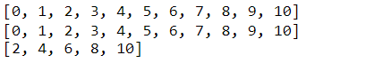

• enumerate(): Another useful built-in function is enumerate. enumerate creates an index item pair for each item in the object provided. For example, calling enumerate on the list of letters produces a sequence of indexed values. Similar to the range function, enumerate returns an enumerate object, which can also be converted into a list and printed.

letters = ['a', 'b', 'c', 'd' ]
indexed_letters = enumerate(letters)
indexed_letters_list = list(indexed_letters)
print(indexed_letters_list)

We can also specify the starting index of enumerate with the keyword argument start. Here, we tell enumerate to start the index at five by passing start equals five into the function call.

#specify a start value
letters = ['a', 'b', 'c', 'd' ]
indexed_letters2 = enumerate(letters, start=5)
indexed_letters2_list = list(indexed_letters2)
print(indexed_letters2_list)

• map(): The last notable built-in function we’ll cover is the map() function. map applies a function to each element in an object. Notice that the map function takes two arguments: first, the function you’d like to apply, and second, the object you’d like to apply that function on. Here, we use a map to apply the built-in function round to each element of the nums list.

nums = [1.5, 2.3, 3.4, 4.6, 5.0]
rnd_nums = map(round, nums)
print(list(rnd_nums))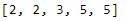

The map function can also be used with a lambda, or an anonymous function. Notice here that we can use the map function and a lambda expression to apply a function, which we’ve defined on the fly, to our original list nums. The map function provides a quick and clean way to apply a function to an object iteratively without writing a for loop.

# map() with lambda 
nums = [1, 2, 3, 4, 5]
sqrd_nums = map(lambda x: x ** 2, nums)
print(list(sqrd_nums))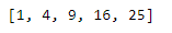

Python Modules

NumPy, or Numerical Python, is an invaluable Python package for Data Scientists. It is the fundamental package for scientific computing in Python and provides a number of benefits for writing efficient code.

NumPy arrays provide a fast and memory-efficient alternative to Python lists. Typically, we import NumPy as np and use np dot to create a NumPy array.

# python list 
nums_list = list(range(5))
print(nums_list)

# using numpyu alternative to python lists
import numpy as np
nums_np = np.array(range(5))
print(nums_np)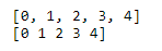

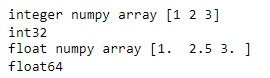
NumPy arrays are homogeneous, which means that they must contain elements of the same type. We can see the type of each element using the .dtype method.

Suppose we created an array using a mixture of types. Here, we create the array nums_np_floats using the integers [1,3] and a float [2.5]. Can you spot the difference in the output? The integers now have a preceding dot in the array.

That’s because NumPy converted the integers to floats to retain that array’s homogeneous nature. Using .dtype, we can verify that the elements in this array are floats.

# NumPy array homogeneity

nums_np_ints = np.array([1, 2, 3]) 
print('integer numpy array',nums_np_ints)
print(nums_np_ints.dtype)

nums_np_floats = np.array([1, 2.5, 3])
print('float numpy array',nums_np_floats)
print(nums_np_floats.dtype)

Homogeneity allows NumPy arrays to be more memory efficient and faster than Python lists. Requiring all elements be the same type eliminates the overhead needed for data type checking.

When analyzing data, you’ll often want to perform operations over entire collections of values quickly. Say, for example, you’d like to square each number within a list of numbers.

It’d be nice if we could simply square the list and get a list of squared values returned. Unfortunately, Python lists don’t support these types of calculations.

# Python lists don't support broadcasting
nums = [-2, -1, 0, 1, 2]
nums ** 2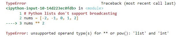

We could square the values using a list by writing a for loop or using a list comprehension, as shown in the code below. But neither of these approaches is the most efficient way of doing this.

Here lies the second advantage of NumPy arrays — their broadcasting functionality. NumPy arrays vectorize operations, so they are performed on all elements of an object at once. This allows us to efficiently perform calculations over entire arrays.

Let's compare the computational time using these three approaches in the following code:

import time

# define numerical list 
nums = range(0,1000)
nums = list(nums)

# For loop (inefficient option)
# get the start time
st = time.time()

sqrd_nums = []
for num in nums:
    sqrd_nums.append(num ** 2)
#print(sqrd_nums)

# get the end time
et = time.time()

# get the execution time
elapsed_time = et - st
print('Execution time using for loops over list:', elapsed_time, 'seconds')


# List comprehension (better option but not best)
# get the start time
st = time.time()

sqrd_nums = [num ** 2 for num in nums]
#print(sqrd_nums)

# get the end time
et = time.time()
print('Execution time using list comprehension:', elapsed_time, 'seconds')


# using numpy array broadcasting

# define the numpy array 
nums_np = np.arange(0,1000)
# get the start time
st = time.time()

nums_np ** 2

# get the end time
et = time.time()

# get the execution time
elapsed_time = et - st
print('Execution time using numpy array broadcasting:', elapsed_time, 'seconds')

We can see that the first two approaches have the same time complexity, while using NumPy in the third approach has decreased the computational time by half.

Another advantage of NumPy arrays is their indexing capabilities. When comparing basic indexing between a one-dimensional array and a list, the capabilities are identical. When using two-dimensional arrays and lists, the advantages of arrays are clear.

To return the second item of the first row in our two-dimensional object, the array syntax is [0,1]. The analogous list syntax is a bit more verbose, as you have to surround both the zero and one with square brackets [0][1].

To return the first column values in the 2-d object, the array syntax is [:,0]. Lists don’t support this type of syntax, so we must use a list comprehension to return columns.

#2-D list
nums2 = [ [1, 2, 3],
        [4, 5, 6] ]


# 2-D array
nums2_np = np.array(nums2)

# printing the second item of the first row 
print(nums2[0][1])
print(nums2_np[0,1])

# printing the first row values 

print([row[0] for row in nums2])
print(nums2_np[:,0])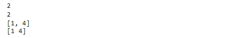

NumPy arrays also have a special technique called boolean indexing. Suppose we wanted to gather only positive numbers from the sequence listed here.

With an array, we can create a Boolean mask using a simple inequality. Indexing the array is as simple as enclosing this inequality in square brackets.

However, to do this using a list, we need to write a for loop to filter the list or use a list comprehension. In either case, using a NumPy array as the index is less verbose and has a faster runtime.

nums = [-2, -1, 0, 1, 2]
nums_np = np.array(nums)

# Boolean indexing
print(nums_np[nums_np > 0])

# No boolean indexing for lists
# For loop (inefficient option)


pos = []
for num in nums:
    if num > 0:
        pos.append(num)
print(pos)


# List comprehension (better option but not best)
pos = [num for num in nums if num > 0]
print(pos)

---

2. Python Code Timing and Profiling

In the second section of the article, you will learn how to gather and compare runtimes between different coding approaches. You’ll practice using the line_profiler and memory_profiler packages to profile your code base and spot bottlenecks. Then, you’ll put your learnings into practice by replacing these bottlenecks with efficient Python code.

2.1. Python Runtime Investigation

As mentioned in the previous section, code efficiency means fast code. To be able to measure how fast our code is, we need to be able to measure the code's runtime.

Comparing runtimes between two code bases that effectively do the same thing allows us to pick the code with the optimal performance. By gathering and analyzing runtimes, we can be sure to implement the code that is fastest and thus more efficient.

To compare runtimes, we need to be able to compute the runtime for a line or multiple lines of code. IPython comes with some handy built-in magic commands we can use to time our code.

Magic commands are enhancements that have been added on top of the normal Python syntax. These commands are prefixed with the percentage sign. If you aren’t familiar with magic commands, take a moment to review the documentation.

Let's start with this example: we want to inspect the runtime for selecting 1,000 random numbers between zero and one using NumPy’s random.rand() function. Using %timeit just requires adding the magic command before the line of code we want to analyze. That’s it! One simple command to gather runtimes.

%timeit rand_nums = np.random.rand(1000)

As we can see, %timeit provides an average of timing statistics. This is one of the advantages of using %timeit. We also see that multiple runs and loops were generated. %timeit runs through the provided code multiple times to estimate the code’s average execution time.

This provides a more accurate representation of the actual runtime rather than relying on just one iteration to calculate the runtime. The mean and standard deviation displayed in the output are a summary of the runtime considering each of the multiple runs.

The number of runs represents how many iterations you’d like to use to estimate the runtime. The number of loops represents how many times you’d like the code to be executed per run.

We can specify the number of runs, using the -r flag, and the number of loops, using the -n flag. Here, we use -r2 to set the number of runs to two and -n10 to set the number of loops to ten. In this example, %timeit would execute our random number selection 20 times in order to estimate the runtime (2 runs each with 10 executions).

# Set number of runs to 2 (-r2)
# Set number of loops to 10 (-n10)
%timeit -r2 -n10 rand_nums = np.random.rand(1000)

Another cool feature of %timeit is its ability to run on single or multiple lines of code. When using %timeit in line magic mode, or with a single line of code, one percentage sign is used, and we can run %timeit in cell magic mode (or provide multiple lines of code) by using two percentage signs.

%%timeit
# Multiple lines of code
nums = []
for x in range(10):
    nums.append(x)

We can also save the output of %timeit into a variable using the -o flag. This allows us to dig deeper into the output and see things like the time for each run, the best time for all runs, and the worst time for all runs.

# Saving the output to a variable and exploring them

times = %timeit -o rand_nums = np.random.rand(1000)
print('The timings for all the 7 runs',times.timings)
print('The best timing is',times.best)
print('The worst timeing is',times.worst)

2.2. Code profiling for runtime

We’ve covered how to time the code using the magic command %timeit, which works well with bite-sized code. But what if we wanted to time a large code base or see the line-by-line runtimes within a function? In this section, we’ll cover a concept called code profiling that allows us to analyze code more efficiently.

Code profiling is a technique used to describe how long and how often various parts of a program are executed. The beauty of a code profiler is its ability to gather summary statistics on individual pieces of our code without using magic commands like %timeit.

We’ll focus on the line_profiler package to profile a function’s runtime line-by-line. Since this package isn’t a part of Python’s Standard Library, we need to install it separately. This can easily be done with a pip install command, as shown in the code below.

!pip install line_profiler

Let’s explore using line_profiler with an example. Suppose we have a list of names along with each person's height (in centimeters) and weight (in kilograms) loaded as NumPy arrays.

names = ['Ahmed', 'Mohammed', 'Youssef']
hts = np.array([188.0, 191.0, 185.0])
wts = np.array([ 95.0, 100.0, 75.0])

We will then develop a function called convert_units that converts each person’s height from centimeters to inches and weight from kilograms to pounds.

def convert_units(names, heights, weights):
    new_hts = [ht * 0.39370 for ht in heights]
    new_wts = [wt * 2.20462 for wt in weights]
    data = {}
    for i,name in enumerate(names):
        data[name] = (new_hts[i], new_wts[i])
    return data
convert_units(names, hts, wts)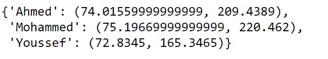

If we wanted to get an estimated runtime of this function, we could use %timeit. But this will only give us the total execution time. What if we wanted to see how long each line within the function took to run? One solution is to use %timeit on each individual line of our convert_units function. But that’s a lot of manual work and not very efficient.

%timeit convert_units(names, hts, wts)

Instead, we can profile our function with the line_profiler package. To use this package, we first need to load it into our session. We can do this using the command %load_ext followed by line_profiler.

%load_ext line_profiler

Now, we can use the magic command %lprun, from line_profiler, to gather runtimes for individual lines of code within the convert_units function. %lprun uses a special syntax. First, we use the -f flag to indicate we’d like to profile a function.

Then, we specify the name of the function we’d like to profile. Note, the name of the function is passed without any parentheses. Finally, we provide the exact function call we’d like to profile by including any arguments that are needed. This is shown in the code below:

%lprun -f convert_units convert_units(names, hts, wts)

The output from %lprun provides a nice table that summarizes the profiling statistics, as shown below. The first column (called Line ) specifies the line number, followed by a column displaying the number of times that line was executed (called the Hits column).

Next, the Time column shows the total amount of time each line took to execute. This column uses a specific timer unit that can be found in the first line of the output.

Here, the timer unit is listed in 0.1 microseconds using scientific notation. We see that line two took 362 timer units, or roughly 36.2 microseconds to run. The Per Hit column gives the average amount of time spent executing a single line.

This is calculated by dividing the Time column by the Hits column. Notice that line 6 was executed three times and had a total run time of 15.4 microseconds, 5 microseconds per hit.

The % Time column shows the percentage of time spent on a line relative to the total amount of time spent in the function. This can be a nice way to see which lines of code are taking up the most time within a function. Finally, the source code is displayed for each line in the Line Contents column.

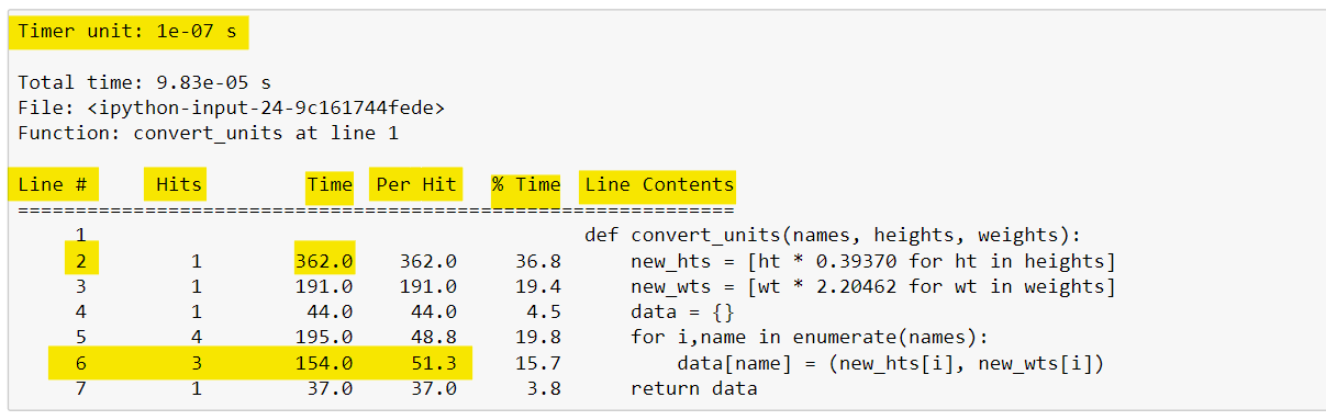
It is noteworthy to mention that the Total time reported when using %lprun and the time reported from using %timeit do not match. Remember, %timeit uses multiple loops in order to calculate an average and standard deviation of time, so the time reported from each of these magic commands isn’t expected to match exactly.

2.3. Code profiling for memory use

We’ve defined efficient code as code that has a minimal runtime and a small memory footprint. So far, we’ve only covered how to inspect the runtime of our code. In this section, we’ll cover a few techniques on how to evaluate our code’s memory usage.

One basic approach for inspecting memory consumption is using Python’s built-in module sys. This module contains system-specific functions and contains one nice method .getsizeof, which returns the size of an object in bytes. sys.getsizeof() is a quick way to see the size of an object.

import sys
nums_list = [*range(1000)]
sys.getsizeof(nums_list)

nums_np = np.array(range(1000))
sys.getsizeof(nums_np)

We can see that the memory allocation of a list is almost double that of a NumPy array. However, this method only gives us the size of an individual object. However, if we wanted to inspect the line-by-line memory size of our code.

As the runtime profile, we could use a code profiler. Just like we’ve used code profiling to gather detailed stats on runtimes, we can also use code profiling to analyze the memory allocation for each line of code in our code base.

We’ll use the memory_profiler package, which is very similar to the line_profiler package. It can be downloaded via pip and comes with a handy magic command (%mprun) that uses the same syntax as %lprun.

!pip install memory_profiler

To be able to apply %mprun to a function and calculate the meomery allocation, this function should be loaded from a separate physical file and not in the IPython console, so first we will create a utils_funcs.py file and define the convert_units function in it, and then we will load this function from the file and apply %mprun to it.

from utils_funcs import convert_units

%load_ext memory_profiler
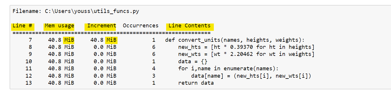
%mprun -f convert_units convert_units(names, hts, wts)

The %mprun output is similar to the %lprun output. In the figure below, we can see a line-by-line description of the memory consumption for the function in question.

The first column represents the line number of the code that has been profiled. The second column (Mem usage) is the memory used after that line has been executed.

Next, the Increment column shows the difference in memory of the current line with respect to the previous one. This shows us the impact of the current line on total memory usage.

Then the occurrence column defines the number of occurrences of this line. The last column (Line Contents) shows the source code that has been profiled.

Profiling a function with %mprun allows us to see what lines are taking up a large amount of memory and possibly develop a more efficient solution.

Important remark

It is noteworthy to mention that memory is reported in mebibytes. Although one mebibyte is not exactly the same as one megabyte, for our purposes, we can assume they are close enough to mean the same thing. Another worth noting is that the memory_profiler package inspects memory consumption by querying the operating system.

This might be slightly different from the amount of memory that is actually used by the Python interpreter. Thus, results may differ between platforms and even between runs. Regardless, the important information can still be observed.

---

In this article, we discussed what efficient Python code then we discussed and explored some of the most important Python built-in standard libraries. After that, we discussed how to measure your code efficiency. In the next article, we will discuss how to optimize your code based on the efficiency measurement we discussed in this article.

3. References

1. https://github.com/youssefHosni/Advanced-Python-Programming-Tutorials-

2. https://app.datacamp.com/learn/courses/writing-efficient-python-code

---

Are you looking to start a career in data science and AI, but do not know how? I offer data science mentoring sessions and long-term career mentoring:

• Mentoring sessions: https://lnkd.in/dXeg3KPW

• Long-term mentoring: https://lnkd.in/dtdUYBrM