Efficient Python for Data Scientists Course [7/14]: Best Practices To Use Pandas Efficiently As A Data Scientist

How To Use Pandas Efficiently As A Data Scientist?

As a data scientist, it is important to use the right tools and techniques to get the most out of the data. The Pandas library is a great tool for data manipulation, analysis, and visualization, and it is an essential part of any data scientist’s toolkit.

However, it can be challenging to use Pandas efficiently, and this can lead to wasted time and effort. Fortunately, there are a few best practices that can help data scientists get the most out of their Pandas experience.

From using vectorized operations to taking advantage of built-in functions, these best practices will help data scientists quickly and accurately analyze and visualize data using Pandas. Understanding and applying these best practices will help data scientists increase their productivity and accuracy, allowing them to make better decisions faster.

Photo by Sid Balachandran on Unsplash

Table of Contents:

1. Why do we need Efficient Coding?

2. Selecting & Replacing Values Effectively
   2.1. Selecting Rows & Columns Efficiently using .iloc[] & .loc[]
   2.2. Replacing Values in a DataFrame Effectively
   2.3. Summary of best practices for selecting and replacing values

3. Iterate Effectively Through Pandas DataFrame
   3.1. Looping effectively using the .iterrows()
   3.2. Looping effectively using .apply()
   3.3. Looping effectively using vectorization
   3.4. Summary of best practices for looping through DataFrame

4. Transforming Data Effectively With .groupby()
   4.1. Common functions used with .groupby()
   4.2. Missing value imputation using .groupby() & .transform()
   4.3. Data filtration using the .groupby() & .filter()

5. Summary of Best Practices

Throughout this article, we will use three datasets:

• Poker card game dataset

• Popular baby names

• Restaurant dataset

The first dataset is the Poker card game dataset, which is shown below:

poker_data = pd.read_csv(’poker_hand.csv’)
poker_data.head()

In each poker round, each player has five cards in hand, each one characterized by its symbol, which can be either hearts, diamonds, clubs, or spades, and its rank, which ranges from 1 to 13. The dataset consists of every possible combination of five cards that one person can possess.

• Sn: symbol of the n-th card where: 1 (Hearts), 2 (Diamonds), 3 (Clubs), 4 (Spades)

• Rn: rank of the n-th card where: 1 (Ace), 2–10, 11 (Jack), 12 (Queen), 13 (King)

The second dataset we will work with is the Popular baby names dataset, which includes the most popular names that were given to newborns between 2011 and 2016. The dataset is loaded and shown below:

names = pd.read_csv(’Popular_Baby_Names.csv’)
names.head()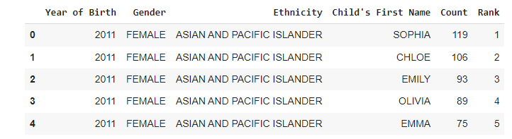

The dataset includes, among other information, the most popular names in the US by year, gender, and ethnicity. For example, the name Chloe was ranked second in popularity among all female newborns of Asian and Pacific Islander ethnicity in 2011.

The third dataset we will use is the Restaurant dataset. This dataset is a collection of people having dinner at a restaurant. The dataset is loaded and shown below:

restaurant = pd.read_csv(’restaurant_data.csv’)
restaurant.head()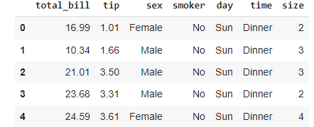

For each customer, we have various characteristics, including the total amount paid, the tips left to the waiter, the day of the week, and the time of the day.

---

---

1. Why do we need Efficient Coding?

Efficient code is code that executes faster and with lower computational meomery. In this article, we will use the time() function to measure the computational time.

This function measures the current time, so we will assign it to a variable before the code execution and after, and then calculate the difference to know the computational time of the code. A simple example is shown in the code below:

import time

# record time before execution
start_time = time.time()

# execute operation
result = 5 + 2

# record time after execution
end_time = time.time()

print(”Result calculated in {} sec”.format(end_time - start_time))

Let’s see some examples of how applying efficient code methods will improve the code runtime and decrease the computational time complexity: We will calculate the square of each number from zero up to a million. At first, we will use a list comprehension to execute this operation, and then repeat the same procedure using a for loop.

First, using list comprehension:

#using List comprehension 

list_comp_start_time = time.time()
result = [i*i for i in range(0,1000000)]
list_comp_end_time = time.time()
print(”Time using the list_comprehension: {} sec”.format(list_comp_end_time -
list_comp_start_time))

Now we will use a for loop to execute the same operation:

# Using For loop

for_loop_start_time= time.time()
result=[]
for i in range(0,1000000):
  result.append(i*i)

for_loop_end_time= time.time()
print(”Time using the for loop: {} sec”.format(for_loop_end_time - for_loop_start_time))

We can see that there is a big difference between them. We can calculate the difference between them in percentage:

list_comp_time = list_comp_end_time - list_comp_start_time
for_loop_time = for_loop_end_time - for_loop_start_time
print(”Difference in time: {} %”.format((for_loop_time - list_comp_time)/ list_comp_time*100))

Here is another example to show the effect of writing efficient code. We would like to calculate the sum of all consecutive numbers from 1 to 1 million. There are two ways: the first is to use brute force, in which we will add one by one to a million.

def sum_brute_force(N):
  res = 0
  for i in range(1,N+1):
    res+=i
  return res

# Using brute force
bf_start_time = time.time()
bf_result = sum_brute_force(1000000)
bf_end_time = time.time()

print(”Time using brute force: {} sec”.format(bf_end_time - bf_start_time))

Another more efficient method is to use a formula to calculate it. When we want to calculate the sum of all the integer numbers from 1 up to a number, let’s say N, we can multiply N by N+1, and then divide by 2, and this will give us the result we want.

This problem was actually given to some students back in Germany in the 19th century, and a bright student called Carl-Friedrich Gauss devised this formula to solve the problem in seconds.

def sum_formula(N):
  return N*(N+1)/2
  
# Using the formula
formula_start_time = time.time()
formula_result = sum_formula(1000000)
formula_end_time = time.time()

print(”Time using the formula: {} sec”.format(formula_end_time - formula_start_time))

After running both methods, we achieve a massive improvement with a magnitude of over 160,000%, which clearly demonstrates why we need efficient and optimized code, even for simple tasks.

---

2. Selecting & Replacing Values Effectively

Let’s first start with two of the most common tasks that you will commonly do on your DataFrame, especially in the data manipulation phase of a data science project.

These two tasks are selecting specific and random rows and columns efficiently, and the usage of the replace() function for replacing one or multiple values using lists and dictionaries

2.1. Selecting Rows & Columns Efficiently using .iloc[ ] & .loc[ ]

In this subsection, we will introduce how to locate and select rows efficiently from dataframes using .iloc[] & .loc[] pandas functions. We will use iloc[] for the index number locator and loc[] for the index name locator.

In the example below, we will select the first 500 rows of the poker dataset. Firstly, by using the .loc[] function, and then by using the .iloc[] function.

# Specify the range of rows to select
rows = range(0, 500)

# Time selecting rows using .loc[]
loc_start_time = time.time()
poker_data.loc[rows]
loc_end_time = time.time()

print(”Time using .loc[] : {} sec”.format(loc_end_time - loc_start_time))

# Specify the range of rows to select
rows = range(0, 500)

# Time selecting rows using .iloc[]
iloc_start_time = time.time()
poker_data.iloc[rows]
iloc_end_time = time.time()

print(”Time using .iloc[]: {} sec”.format(iloc_end_time - iloc_start_time))

loc_comp_time = loc_end_time - loc_start_time
iloc_comp_time = iloc_end_time - iloc_start_time

print(”Difference in time: {} %”.format((loc_comp_time - iloc_comp_time)/ iloc_comp_time*100))

While these two methods have the same syntax, iloc[] performs almost 70% faster than loc[]. The .iloc[] function takes advantage of the order of the indices, which are already sorted, and is therefore faster.

We can also use them to select columns, not only rows. In the next example, we will select the first three columns using both methods.

iloc_start_time = time.time()

poker_data.iloc[:,:3]
iloc_end_time = time.time()

print(”Time using .iloc[]: {} sec”.format(iloc_end_time - iloc_start_time))

names_start_time = time.time()
poker_data[[’S1’, ‘R1’, ‘S2’]]
names_end_time = time.time()

print(”Time using selection by name: {} sec”.format(names_end_time - names_start_time))

loc_comp_time = names_end_time - names_start_time
iloc_comp_time = iloc_end_time - iloc_start_time
print(”Difference in time: {} %”.format((loc_comp_time - iloc_comp_time)/
loc_comp_time*100))

We can also see that using column indexing using iloc[] is still 80% faster. So it is better to use iloc[] as it is faster unless it is easier to use the loc[] to select certain columns by name.

2.2. Replacing Values in a DataFrame Effectively

Replacing values in a DataFrame is a very important task, especially in the data cleaning phase. Since you will have to keep the whole values that represent the same object, the same.

Let’s take a look at the popular baby names dataset we loaded before:

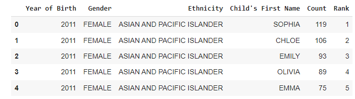
Let’s have a closer look at the Gender feature and see the unique values they have:

names[’Gender’].unique()

We can see that the female gender is represented with two values, both uppercase and lowercase. This is very common in real data, and an easy way to do so is to replace one of the values with the other to keep it consistent throughout the whole dataset.

There are two ways to do it. The first one is simply defining which values we want to replace, and then what we want to replace them with. This is shown in the code below:

start_time = time.time()
names[’Gender’].loc[names.Gender==’female’] = ‘FEMALE’
end_time = time.time()

pandas_time = end_time - start_time
print(”Replace values using .loc[]: {} sec”.format(pandas_time))

The second method is to use the Panda’s built-in function. .replace() as shown in the code below:

start_time = time.time()
names[’Gender’].replace(’female’, ‘FEMALE’, inplace=True)
end_time = time.time()
replace_time = end_time - start_time

print(”Time using replace(): {} sec”.format(replace_time))

We can see that there is a difference in time complexity with the built-in function, 157% faster than using the .loc() method to find the rows and columns index of the values and replace them.

print(’The differnce: {} %’.format((pandas_time- replace_time )/replace_time*100))

We can also replace multiple values using lists. Our objective is to change all ethnicities classified as WHITE NON-HISPANIC or WHITE NON-HISP to WNH. Using the .loc[] function, we will locate babies of the ethnicities we are looking for, using the ‘or’ statement (which in Python is symbolized by the pipe).

We will then assign the new value. As always, we also measure the CPU time needed for this operation.

start_time = time.time()

names[’Ethnicity’].loc[(names[”Ethnicity”] == ‘WHITE NON HISPANIC’) |
(names[”Ethnicity”] == ‘WHITE NON HISP’)] = ‘WNH’

end_time = time.time()
pandas_time= end_time - start_time

print(”Results from the above operation calculated in %s seconds” %(pandas_time))

We can also do the same operation using the .replace() pandas built-in function as follows:

start_time = time.time()
names[’Ethnicity’].replace([’WHITE NON HISPANIC’,’WHITE NON HISP’],
‘WNH’, inplace=True)

end_time = time.time()
replace_time = end_time - start_time

print(”Time using .replace(): {} sec”.format(replace_time))

We can see that again using the .replace() method is much faster than using the .loc[] method. To have a better intuition of how much faster it is, let’s run the code below:

print(’The differnce: {} %’.format((pandas_time- replace_time )/replace_time*100))

The .replace() method is 87% faster than using the .loc[] method. If your data is huge and needs a lot of cleaning, this tip will decrease the computational time of your data cleaning and make your pandas code much faster and hence more efficient.

Finally, we can also use dictionaries to replace both single and multiple values in your DataFrame. This will be very helpful if you would like to replace multiple functions in one command.

We’re going to use dictionaries to replace every male’s gender with BOY and every female’s gender with GIRL.

names = pd.read_csv(’Popular_Baby_Names.csv’)

start_time = time.time()

names[’Gender’].replace({’MALE’:’BOY’, ‘FEMALE’:’GIRL’, ‘female’: ‘girl’}, inplace=True)

end_time = time.time()
dict_time = end_time - start_time

print(”Time using .replace() with dictionary: {} sec”.format(dict_time))

names = pd.read_csv(’Popular_Baby_Names.csv’)

start_time = time.time()

names[’Gender’].replace(’MALE’, ‘BOY’, inplace=True)
names[’Gender’].replace(’FEMALE’, ‘GIRL’, inplace=True)
names[’Gender’].replace(’female’, ‘girl’, inplace=True)

end_time = time.time()

list_time = end_time - start_time
print(”Time using multiple .replace(): {} sec”.format(list_time))

print(’The differnce: {} %’.format((list_time- dict_time )/dict_time*100))

We could do the same thing with lists, but it’s more verbose. If we compare both methods, we can see that dictionaries run approximately 22% faster. In general, working with dictionaries in Python is very efficient compared to lists: looking through a list requires a pass through every element of the list, while looking at a dictionary directs instantly to the key that matches the entry.

The comparison is a little unfair, though, since both structures serve different purposes.

Using dictionaries allows you to replace the same values in several different columns. In all the previous examples, we specified the column from which the values to replace came.

We’re now going to replace several values from the same column with one common value. We want to classify all ethnicities into three big categories: Black, Asian, and White.

The syntax again is very simple. We use nested dictionaries here: the outer key is the column in which we want to replace values. The value of this outer key is another dictionary, where the keys are the ethnicities to replace, and the values for the new ethnicity (Black, Asian, or White).

start_time = time.time()

names.replace({’Ethnicity’: {’ASIAN AND PACI’: ‘ASIAN’, ‘ASIAN AND PACIFIC ISLANDER’: ‘ASIAN’,‘BLACK NON HISPANIC’: ‘BLACK’, ‘BLACK NON HISP’: ‘BLACK’,‘WHITE NON HISPANIC’: ‘WHITE’, ‘WHITE NON HISP’: ‘WHITE’}})

print(”Time using .replace() with dictionary: {} sec”.format (time.time() - start_time))

2.3. Summary of best practices for selecting and replacing values

• Selecting rows and columns is faster using the .iloc[] function. So it is better to use unless it is easier or more convenient to use .loc[], and the speed is not a priority, or you are just doing it once.

• Using the built-in replace() function is much faster than just using conventional methods.

• Replacing multiple values using Python dictionaries is faster than using lists.

---

3. Iterate Effectively Through Pandas DataFrame

As a data scientist, you will need to iterate through your dataframe extensively, especially in the data preparation and exploration phase, so it is important to be able to do this efficiently, as it will save you much time and give space for more important work.

We will walk through three methods to make your loops much faster and more efficient:

• Looping using the .iterrows() function

• Looping using the .apply() function

• Vectorization

3.1. Looping effectively using .iterrows()

Before we talk about how to use the .iterrows() function to improve the looping process, let’s refresh the notion of a generator function.

Generators are a simple tool to create iterators. Inside the body of a generator, instead of return statements, you will find only yield() statements. There can be just one or several yield() statements. Here, we can see a generator, city_name_generator(), that produces four city names. We assign the generator to the variable city_names for simplicity.

def city_name_generator():
  yield(’New York’)
  yield(’London’)
  yield(’Tokyo’)
  yield(’Sao Paolo’)

city_names = city_name_generator()

To access the elements that the generator yields, we can use Python’s next() function. Each time the next() command is used, the generator will produce the next value to yield, until there are no more values to yield. We have 4 cities.

Let’s run the next command four times and see what it returns:

next(city_names)

next(city_names)

next(city_names)

As we can see that every time we run the next() function, it will print a new city name.

Let’s go back to the .iterrows() function. The .iterrows() function is a property of every pandas DataFrame. When called, it produces a list with two elements. We will use this generator to iterate through each line of our poker DataFrame.

The first element is the index of the row, while the second element contains a pandas Series of each feature of the row: the Symbol and the Rank for each of the five cards. It is very similar to the notion of the enumerate() function, which, when applied to a list, returns each element along with its index.

The most intuitive way to iterate through a Pandas DataFrame is to use the range() function, which is often called crude looping. This is shown with the code below:

start_time = time.time()
for index in range(poker_data.shape[0]):
  next

print(”Time using range(): {} sec”.format(time.time() - start_time))

One smarter way to iterate through a pandas DataFrame is to use the .iterrows() function, which is optimized for this task. We simply define the ‘for’ loop with two iterators, one for the number of each row and the other for all the values.

Inside the loop, the next() command indicates that the loop moves to the next value of the iterator, without actually doing anything.

data_generator = poker_data.iterrows()
start_time = time.time()

for index, values in data_generator:
  next

print(”Time using .iterrows(): {} sec”.format(time.time() - start_time))

Comparing the two computational times, we can also notice that the use of .iterrows() does not improve the speed of iterating through a pandas DataFrame. It is very useful, though, when we need a cleaner way to use the values of each row while iterating through the dataset.

3.2. Looping effectively using .apply()

Now we will use the .apply() function to be able to perform a specific task while iterating through a pandas DataFrame. The .apply() function does exactly what it says; it applies another function to the whole DataFrame.

The syntax of the .apply() function is simple: we create a mapping, using a lambda function in this case, and then declare the function we want to apply to every cell.

Here, we’re applying the square root function to every cell of the DataFrame. In terms of speed, it matches the speed of just using the NumPy sqrt() function over the whole DataFrame.

data_sqrt = poker_data.apply(lambda x: np.sqrt(x))
data_sqrt.head()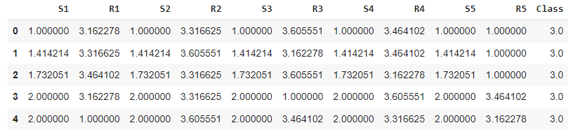

This is a simple example since we would like to apply this function to the dataframe.

But what happens when the function of interest takes more than one cell as an input? For example, what if we want to calculate the sum of the ranks of all the cards in each hand?

In this case, we will use the .apply() function the same way as we did before, but we need to add ‘axis=1’ at the end of the line to specify we’re applying the function to each row.

apply_start_time = time.time()

poker_data[[’R1’, ‘R2’, ‘R3’, ‘R4’, ‘R5’]].apply(lambda x: sum(x), axis=1)

apply_end_time = time.time()

apply_time = apply_end_time - apply_start_time

print(”Time using .apply(): {} sec”.format(time.time() - apply_start_time))

Then, we will use the .iterrows() function we saw previously, and compare their efficiency.

for_loop_start_time = time.time()

for ind, value in poker_data.iterrows():
  sum([value[1], value[3], value[5], value[7], value[9]])

for_loop_end_time = time.time()

for_loop_time = for_loop_end_time - for_loop_start_time

print(”Time using .iterrows(): {} sec”.format(for_loop_time))

Using the .apply() function is significantly faster than the .iterrows() function, with a magnitude of around 400 percent, which is a massive improvement!

print(’The differnce: {} %’.format((for_loop_time - apply_time) / apply_time * 100))

As we did with rows, we can do the same thing for the columns; apply one function to each column. By replacing the axis=1 with axis=0, we can apply the sum function on every column.

apply_start_time = time.time()
poker_data[[’R1’, ‘R2’, ‘R3’, ‘R4’, ‘R5’]].apply(lambda x: sum(x), axis=0)
apply_end_time = time.time()
apply_time = apply_end_time - apply_start_time
print(”Time using .apply(): {} sec”.format(apply_time))

By comparing the .apply() function with the native pandas’ function for summing over rows, we can see that pandas’ native .sum() functions perform the same operation faster.

pandas_start_time = time.time()
poker_data[[’R1’, ‘R1’, ‘R3’, ‘R4’, ‘R5’]].sum(axis=0)
pandas_end_time = time.time()
pandas_time = pandas_end_time - pandas_start_time
print(”Time using pandas: {} sec”.format(pandas_time))

print(’The differnce: {} %’.format((apply_time - pandas_time) / pandas_time * 100))

In conclusion, we observe that the .apply() function performs faster when we want to iterate through all the rows of a pandas DataFrame, but is slower when we perform the same operation through a column.

3.3. Looping effectively using vectorization

To understand how we can reduce the amount of iteration performed by the function, recall that the fundamental units of Pandas, DataFrames, and Series, are both based on arrays.

Pandas perform more efficiently when an operation is performed on a whole array than to each value separately or sequentially. This can be achieved through vectorization. Vectorization is the process of executing operations on entire arrays.

In the code below, we want to calculate the sum of the ranks of all the cards in each hand. In order to do that, we slice the poker dataset, keeping only the columns that contain the ranks of each card.

Then, we call the built-in. .sum() property of the DataFrame, using the parameter axis = 1 to denote that we want the sum for each row. In the end, we print the sum of the first five rows of the data.

start_time_vectorization = time.time()

poker_data[[’R1’, ‘R2’, ‘R3’, ‘R4’, ‘R5’]].sum(axis=1)
end_time_vectorization = time.time()

vectorization_time = end_time_vectorization  - start_time_vectorization
print(”Time using pandas vectorization: {} sec”.format(vectorization_time))

We saw previously various methods that perform functions applied to a DataFrame faster than simply iterating through all the rows of the DataFrame. Our goal is to find the most efficient method to perform this task.

• Using .iterrows() to loop through the DataFrame:

  data_generator = poker_data.iterrows()
  
  start_time_iterrows = time.time()
  
  for index, value in data_generator:
    sum([value[1], value[3], value[5], value[7]])
  
  end_time_iterrows = time.time()
  iterrows_time = end_time_iterrows - start_time_iterrows
  print(”Time using .iterrows() {} seconds “ .format(iterrows_time)) 

• Using the .apply() mehtod:

  start_time_apply = time.time()
  poker_data[[’R1’, ‘R2’, ‘R3’, ‘R4’, ‘R5’]].apply(lambda x: sum(x),axis=1)
  end_time_apply = time.time()
  
  apply_time = end_time_apply - start_time_apply
  
  print(”Time using apply() {} seconds”  .format(apply_time))

Comparing the time it takes to sum the ranks of all the cards in each hand using vectorization, the .iterrows() function, and the .apply() function, we can see that the vectorization method performs much better.

We can also use another vectorization method to effectively iterate through the DataFrame, which uses Numpy arrays to vectorize the DataFrame.

The NumPy library, which defines itself as a “fundamental package for scientific computing in Python”, performs operations under the hood in optimized, pre-compiled C code.

Similar to pandas working with arrays, NumPy operates on arrays called ndarrays. A major difference between Series and ndarrays is that ndarrays leave out many operations, such as indexing, data type checking, etc.

As a result, operations on NumPy arrays can be significantly faster than operations on pandas Series. NumPy arrays can be used in place of the pandas Series when the additional functionality offered by the pandas Series isn’t critical.

For the problems we explore in this article, we could use NumPy ndarrays instead of pandas series. The question at stake is whether this would be more efficient or not.

Again, we will calculate the sum of the ranks of all the cards in each hand. We convert our rank arrays from pandas Series to NumPy arrays simply by using the .values method of pandas Series, which returns a pandas Series as a NumPy ndarray.

As with vectorization on the series, passing the NumPy array directly into the function will lead pandas to apply the function to the entire vector.

start_time = time.time()

poker_data[[’R1’, ‘R2’, ‘R3’, ‘R4’, ‘R5’]].values.sum(axis=1)

print(”Time using NumPy vectorization: {} sec” .format(time.time() - start_time))

start_time = time.time()
poker_data[[’R1’, ‘R2’, ‘R3’, ‘R4’, ‘R5’]].sum(axis=1)
print(”Results from the above operation calculated in %s seconds” % (time.time() - start_time))

At this point, we can see that vectorizing over the pandas series achieves the overwhelming majority of optimization needs for everyday calculations.

However, if speed is of the highest priority, we can call in reinforcements in the form of the NumPy Python library. Compared to the previous state-of-the-art method, the panda’s optimization, we still get an improvement in the operating time.

3.4. Summary of best practices for looping through DataFrame

• Using .iterrows() does not improve the speed of iterating through the DataFrame, but it is more efficient.

• The .apply() function performs faster when we want to iterate through all the rows of a pandas DataFrame, but is slower when we perform the same operation through a column.

• Vectorizing over the pandas series achieves the overwhelming majority of optimization needs for everyday calculations. However, if speed is of the highest priority, we can call in reinforcements in the form of the NumPy Python library.

---

4. Transforming Data Effectively With .groupby()

In this last section of the article, we will discuss how to use the .groupby() function effectively to group the entries of a DataFrame according to the values of a specific feature.

The .groupby() method is applied to a DataFrame and groups it according to a feature. Then, we can apply some simple or more complicated functions on that grouped object.

This is a very important tool for every data scientist working on tabular or structured data, as it will help you to manipulate data easily and in a more effective way.

4.1. Common functions used with .groupby()

One of the simplest methods to apply to an aggregated group is the .count(). In the example below, we will apply this to the restaurant dataset.

At first, we group the restaurant data according to whether the customer was a smoker or not. Then, we apply the .count() method. We obtain the count of smokers and non-smokers.

restaurant = pd.read_csv(’restaurant_data.csv’)

restaurant_grouped = restaurant.groupby(’smoker’)
print(restaurant_grouped.count())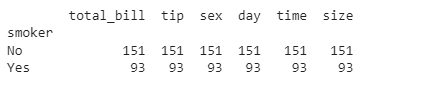

It is no surprise that we get the same results for all the features, as the .count() method counts the number of occurrences of each group in each feature. As there are no missing values in our data, the results should be the same in all columns.

After grouping the entries of the DataFrame according to the values of a specific feature, we can apply any kind of transformation we are interested in.

Here, we are going to apply the z score, a normalization transformation, which is the distance between each value and the mean, divided by the standard deviation.

This is a very useful transformation in statistics, often used with the z-test in standardized testing. To apply this transformation to the grouped object, we just need to call the .transform() method containing the lambda transformation we defined.

This time, we will group according to the type of meal: was it a dinner or a lunch? As the z-score transformation is group-related, the resulting table is just the original table.

For each element, we subtract the mean and divide it by the standard deviation of the group it belongs to. We can also see that numerical transformations are applied only to numerical features of the DataFrame.

zscore = lambda x: (x - x.mean() ) / x.std()

restaurant_grouped = restaurant.groupby(’time’)

restaurant_transformed = restaurant_grouped.transform(zscore)
restaurant_transformed.head()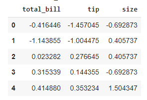

While the transform() method simplifies things a lot, is it actually more efficient than using native Python code? As we did before, we first group our data, this time according to sex.

Then we apply the z-score transformation we applied before, measuring its efficiency. We omit the code for measuring the time of each operation here, as you are already familiar with this.

We can see that with the use of the transform() function, we achieve a massive speed improvement. On top of that, we’re only using one line to operate against interest.

restaurant.groupby(’sex’).transform(zscore)

mean_female = restaurant.groupby(’sex’).mean()[’total_bill’][’Female’]
mean_male = restaurant.groupby(’sex’).mean()[’total_bill’][’Male’]
std_female = restaurant.groupby(’sex’).std()[’total_bill’][’Female’]
std_male = restaurant.groupby(’sex’).std()[’total_bill’][’Male’]

for i in range(len(restaurant)):

  if restaurant.iloc[i][2] == ‘Female’:
    restaurant.iloc[i][0] = (restaurant.iloc[i][0] - mean_female)/std_female
  
  else:
    restaurant.iloc[i][0] = (restaurant.iloc[i][0] - mean_male)/std_male

4.2. Missing value imputation using .groupby() & .transform( )

Now that we have seen why and how to use the transform() function on a grouped pandas object, we will address a very specific task that is imputing missing values.

Before we actually see how we can use the transform() function for missing value imputation, we will see how many missing values there are in our variable of interest in each of the groups. We can see below the number of data points in each of the “time” features, and they are 176+68 = 244.

prior_counts = restaurant.groupby(’time’)
prior_counts[’total_bill’].count()

Next, we will create a restaurant_nan dataset, in which the total bill of 10% random observations was set to NaN using the code below:

import pandas as pd
import numpy as np

p = 0.1 #percentage missing data required

mask = np.random.choice([np.nan,1], size=len(restaurant), p=[p,1-p])
restaurant_nan = restaurant.copy()
restaurant_nan[’total_bill’] =  restaurant_nan[’total_bill’] * mask

Now, let’s print the number of data points in each of the “time” features, and we can see that they are now 155+62 = 217. Since the total data points we have are 244, then the missing data points are 24, which is equal to 10%.

prior_counts = restaurant.groupby(’time’)
prior_counts[’total_bill’].count()

After counting the number of missing values in our data, we will show how to fill these missing values with a group-specific function. The most common choices are the mean and the median, and the selection has to do with the skewness of the data.

As we did before, we define a lambda transformation using the fillna() function to replace every missing value with its group average. As before, we group our data according to the time of the meal and then replace the missing values by applying the pre-defined transformation.

# Missing value imputation

missing_trans = lambda x: x.fillna(x.mean())
restaurant_nan_grouped = restaurant_nan.groupby(’time’)[’total_bill’]
restaurant_nan_grouped.transform(missing_trans)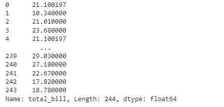

As we can see, the observations at index 0 and index 4 are the same, which means that their missing value has been replaced by their group’s mean.

Also, we can see that the computation time using this method is 0.007 seconds.

Let’s compare this with the conventional method:

start_time = time.time()
mean_din = restaurant_nan.loc[restaurant_nan.time ==’Dinner’][’total_bill’].mean()
mean_lun = restaurant_nan.loc[restaurant_nan.time == ‘Lunch’][’total_bill’].mean()

for row in range(len(restaurant_nan)):
  if restaurant_nan.iloc[row][’time’] == ‘Dinner’:
    restaurant_nan.loc[row, ‘total_time’] = mean_din
  else:
    restaurant_nan.loc[row, ‘total_time’] = mean_lun

print(”Results from the above operation calculated in %s seconds” % (time.time() - start_time))

We can see that using the .transform() function applied to a grouped object performs faster than the native Python code for this task.

4.3. Data filtration using the .groupby() & .filter()

Now we will discuss how we can use the filter() function on a grouped pandas object. This allows us to include only a subset of those groups, based on some specific conditions.

Often, after grouping the entries of a DataFrame according to a specific feature, we are interested in including only a subset of those groups, based on some conditions.

Some examples of filtration conditions are the number of missing values, the mean of a specific feature, or the number of occurrences of the group in the dataset.

We are interested in finding the mean amount of tips given on the days when the mean amount paid to the waiter is more than 20 USD. The .filter() function accepts a lambda function that operates on a DataFrame of each of the groups.

In this example, the lambda function selects “total_bill” and checks that the mean() is greater than 20. If that lambda function returns True, then the mean() of the tip is calculated.

If we compare the total mean of the tips, we can see that there is a difference between the two values, meaning that the filtering was performed correctly.

restaurant_grouped = restaurant.groupby(’day’)
filter_trans = lambda x : x[’total_bill’].mean() > 20
restaurant_filtered = restaurant_grouped.filter(filter_trans)

print(restaurant_filtered[’tip’].mean())

print(restaurant[’tip’].mean())

If we attempt to perform this operation without using groupby(), we end up with this inefficient code. At first, we use a list comprehension to extract the entries of the DataFrame that refer to days that have a mean meal greater than $20, and then use a for loop to append them to a list and calculate the mean. It might seem very intuitive, but as we see, it’s also very inefficient.

t=[restaurant.loc[restaurant[’day’] == i][’tip’] for i in restaurant[’day’].unique()
  if restaurant.loc[restaurant[’day’] == i][’total_bill’].mean()>20]
restaurant_filtered = t[0]

for j in t[1:]:
  restaurant_filtered=restaurant_filtered.append(j,ignore_index=True)

---

5. Summary of Best Practices

• Selecting rows and columns is faster using the .iloc[] function. So it is better to use unless it is easier or more convenient to use .loc[], and the speed is not a priority, or you are just doing it once.

• Using the built-in replace() function is much faster than just using conventional methods.

• Replacing multiple values using Python dictionaries is faster than using lists.

• Using .iterrows() does not improve the speed of iterating through the DataFrame, but it is more efficient.

• The .apply() function performs faster when we want to iterate through all the rows of a pandas DataFrame, but is slower when we perform the same operation through a column.

• Vectorizing over the pandas series achieves the overwhelming majority of optimization needs for everyday calculations. However, if speed is of the highest priority, we can call in reinforcements in the form of the NumPy Python library.

• Using .groupby() to group it according to a certain feature and then using other functions to apply it to the data is much faster than using the conventional coding method.

---

This newsletter is a personal passion project, and your support helps keep it alive. If you would like to contribute, there are a few great ways:

• Subscribe. A paid subscription helps to make my writing sustainable and gives you access to additional content.*

• Grab a copy of my book Bundle. Get my 7 hands-on books and roadmaps for only 40% of the price

Thanks for reading, and for helping support independent writing and research!