
Efficient Python for Data Scientists Course [10/14]: 20 Pandas Functions for 80% of Your Data Science Tasks
Master these Functions and Get Your Work Done

Pandas is one of the most widely used libraries in the data science community, and it’s a powerful tool that can help you with data manipulation, cleaning, and analysis. Whether you’re a beginner or an experienced data scientist, this article will provide valuable insights into the most commonly used Pandas functions and how to use them practically.
We will cover everything from basic data manipulation to advanced data analysis techniques. By the end of this article, you will have a solid understanding of how to use Pandas to make your data science workflow more efficient.

1. pd.read_csv()
pd.read_csv is a function in the pandas library in Python that is used to read a CSV (Comma Separated Values) file and convert it into a pandas DataFrame.
Example:
import pandas as pd
df = pd.read_csv(’Popular_Baby_Names.csv’)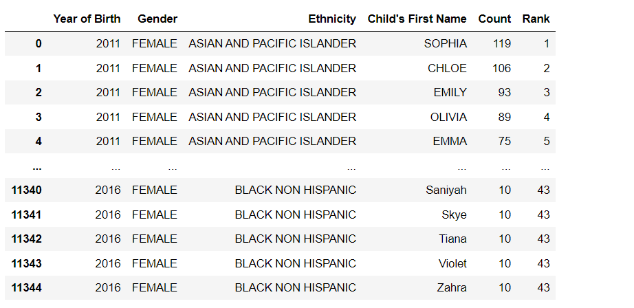
In this example, the pd.read_csv function reads the file ‘data.csv’ and converts it into a DataFrame, which is then assigned to the variable ‘data’. The contents of the DataFrame can then be printed using the print function.
It has many options like sep, header, index_col, skiprows, na_values etc.
df = pd.read_csv(’Popular_Baby_Names.csv’, sep=’;’, header=0, index_col=0, skiprows=5, na_values=’N/A’)This example reads the CSV file data.csv, with ; as a separator, the first row as the header, the first column as an index, skipping the first 5 rows, and replacing N/A with NaN.
2. df.describe()
The df.describe() method in pandas is used to generate summary statistics of various features of a DataFrame. It returns a new DataFrame that contains the count, mean, standard deviation, minimum, 25th percentile, median, 75th percentile, and maximum of each numerical column in the original DataFrame.
print(df.describe())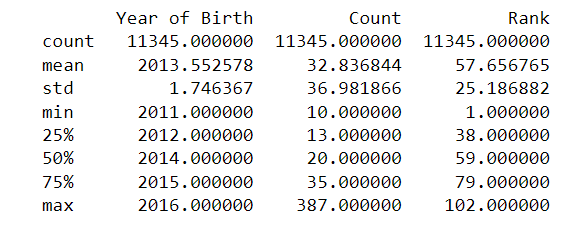
You can also include or exclude certain columns and also include non-numeric columns by passing appropriate arguments to the method.
df.describe(include=’all’) # include all columns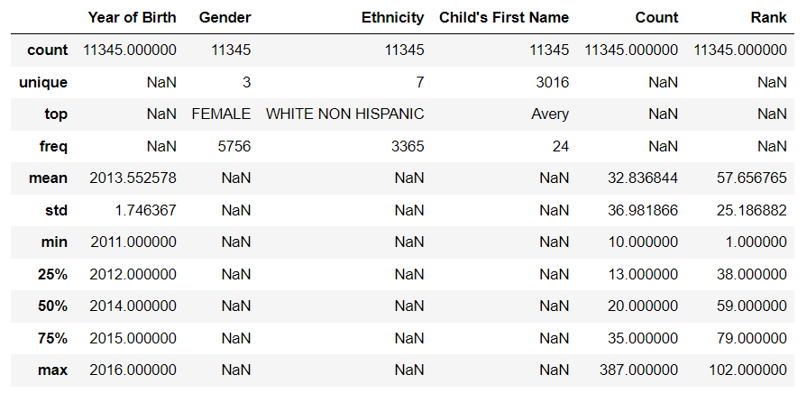
df.describe(exclude=’number’) # exclude numerical columns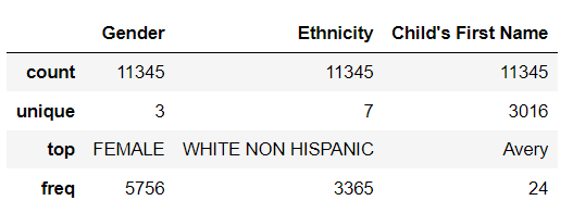
3. df.info()
df.info() is a method in pandas that provides a concise summary of the DataFrame, including the number of non-null values in each column, the data types of each column, and the memory usage of the DataFrame.
print(df.info())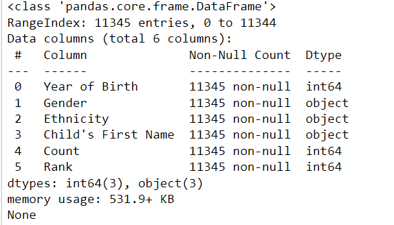
4. df.plot()
df.plot() is a method in pandas that is used to create various types of plots from a DataFrame. By default, it creates a line plot of all numerical columns in the DataFrame. But you can also pass the argument kind to specify the type of plot you want to create. Available options are line, bar, barh, hist, box, kde, density, area, pie, scatter, and hexbin.
In the examples below, I will use the .plot() method to plot numerical and categorical variables. For the categorical variable, I will plot bar and pie plots, and for the numerical variable, I will plot box plots. You can try different types of plots by yourself.
df[’Gender’].value_counts().plot(kind=’bar’)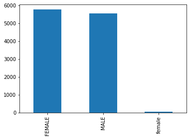
df[’Gender’].value_counts().plot(kind=’pie’)
df[’Count’].plot(kind=’box’)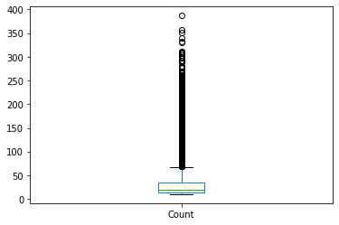
It also supports many other options like title, xlabel, ylabel, legend, grid, xlim, ylim, xticks, yticks etc. to customize the plot. You can also use plt.xlabel(), plt.ylabel(), plt.title() etc., after the plot to customize it.
Please keep in mind that df.plot() is just a convenient wrapper around the matplotlib.pyplot library, so the same customization options are available in matplotlib are available for df.plot().
5. df.iloc()
Pandas’ .iloc() function is used to select rows and columns by their integer-based index in a DataFrame. It is used to select rows and columns by their integer-based location.
Here are some examples of how you can use it:
# Select the first row
print(df.iloc[0])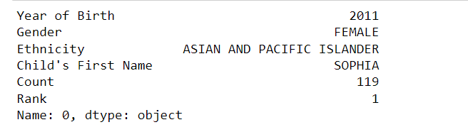
# Select the first two rows
print(df.iloc[:2])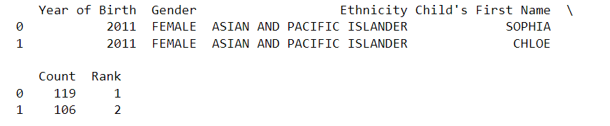
# Select the first column
print(df.iloc[:, 0])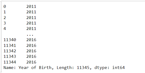
# Select the first two columns
print(df.iloc[:, :2])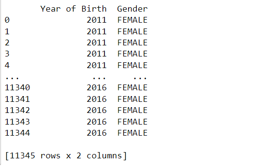
# Select the (1, 1) element
print(df.iloc[1, 1])
In the above examples, df.iloc[0] selects the first row of the dataframe, df.iloc[:2] selects the first two rows, df.iloc[:, 0] selects the first column, df.iloc[:, :2] selects the first two columns, and df.iloc[1, 1] selects the element at the (1, 1) position of the dataframe (second row, second column).
Keep in mind that .iloc() only selects rows and columns based on their integer-based index, so if you want to select rows and columns based on their labels, you should use .loc() method instead, as will be shown next.
6. df.loc()
Pandas’ .loc() function is used to select rows and columns by their label-based index in a DataFrame. It is used to select rows and columns by their label-based location.
Here are some examples of how you can use it:
# Select the column name ‘Gender’
print(df.loc[:,’Gender’])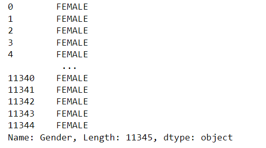
# Select the columns named ‘Year of Birth’ and ‘Gender’
print(df.loc[:, [’Year of Birth’, ‘Gender’]])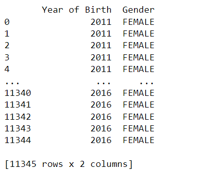
In the above example, we used df.loc[:, ‘Gender’] to selected the column named ‘Gender’, and df.loc[:, [’Year of Birth’, ‘Gender’]] selected the columns named ‘Year of Birth’ and ‘Gender’.
7. df.assign()
Pandas’ .assign() function is used to add new columns to a DataFrame, based on the computation of existing columns. It allows you to add new columns to a DataFrame without modifying the original dataframe. The function returns a new DataFrame with the added columns.
Here is an example of how you can use it:
df_new = df.assign(count_plus_5=df[’Count’] + 5)
df_new.head()
In the above example, the first time df.assign() is used to create a new column named ‘count_plus_5’ with the value of count + 5.
It’s important to note that the original DataFrame df remains unchanged, and the new DataFrame df_new is returned with the new columns added.
The .assign() method can be used multiple times in a chain, allowing you to add multiple new columns to a DataFrame in one line of code.
8. df.query()
Pandas’ .query() function allows you to filter a DataFrame based on a Boolean expression. It allows you to select rows from a DataFrame using a query string similar to SQL. The function returns a new DataFrame containing only the rows that satisfy the Boolean expression.
Here is an example of how you can use it:
# Select rows where age is greater than 30 and income is less than 65000
df_query = df.query(’Count > 30 and Rank < 20’)
df_query.head()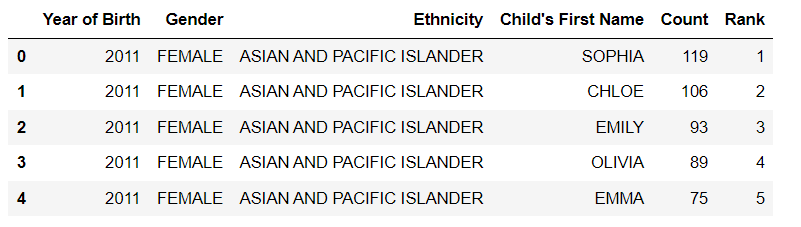
# Select rows where gender is Male
df_query = df.query(”Gender == ‘MALE’”)
df_query.head()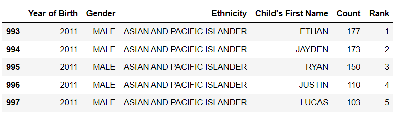
In the above example, the first time df.query() is used to select rows where the count is greater than 30 and the rank is less than 30, and the second time df.query() is used to select rows where gender is ‘MALE’.
It’s important to note that the original DataFrame df remains unchanged, and the new DataFrame df_query is returned with the filtered rows.
The .query() method can be used with any valid Boolean expression, and it’s useful when you want to filter a DataFrame based on multiple conditions or when the conditions are complex and hard to express using the standard indexing operators.
Also, keep in mind that the .query() method is slower than Boolean indexing, so if performance is critical, you should use Boolean indexing instead.
9. df.sort_values()
Pandas’ .sort_values() function allows you to sort a DataFrame by one or multiple columns. It sorts the DataFrame based on the values of one or more columns, in ascending or descending order. The function returns a new DataFrame sorted by the specified column(s).
Here is an example of how you can use it:
# Sort by age in ascending order
df_sorted = df.sort_values(by=’Count’)
df_sorted.head()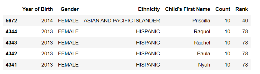
# Sort by income in descending order
df_sorted = df.sort_values(by=’Rank’, ascending=False)
df_sorted.head()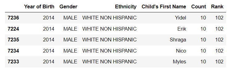
# Sort by multiple columns
df_sorted = df.sort_values(by=[’Count’, ‘Rank’])
df_sorted.head()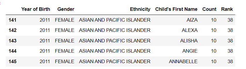
In the above example, the first time df.sort_values() is used to sort the DataFrame by ‘Count’ in ascending order, the second time is used to sort by ‘Rank’ in descending order, and the last time it’s used to sort by multiple columns ‘Count’ and ‘Rank’.
It’s important to note that the original DataFrame df remains unchanged, and the new DataFrame df_sorted is returned with the sorted values.
The .sort_values() method can be used with any column(s) of the DataFrame, and it’s useful when you want to sort the DataFrame based on multiple columns, or when you want to sort the DataFrame by a column in descending order.
10. df.sample()
Pandas’ .sample() function allows you to randomly select rows from a DataFrame. It returns a new DataFrame containing the randomly selected rows. The function takes several parameters that allow you to control the sampling process, such as the number of rows to return, and whether or not to sample with replacement and seed for reproducibility.
Here is an example of how you can use it:
# Sample 2 rows without replacement
df_sample = df.sample(n=2, replace=False, random_state=1)
df_sample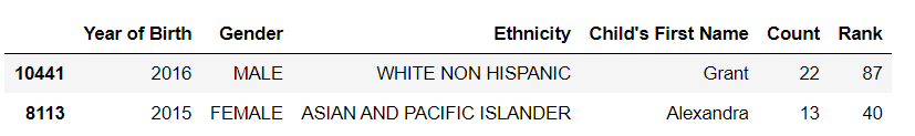
# Sample 3 rows with replacement
df_sample = df.sample(n=3, replace=True, random_state=1)
df_sample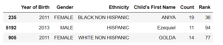
# Sample 2 rows without replacement with specific column to be chosen
df_sample = df.sample(n=2, replace=False, random_state=1, axis=1)
df_sample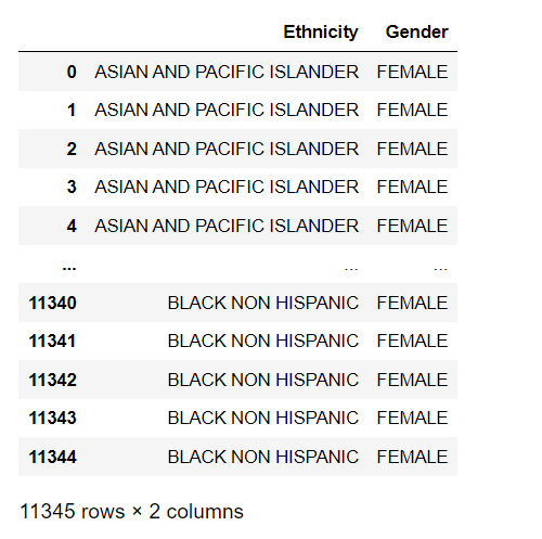
In the above example, the first time df.sample() is used to randomly select 2 rows without replacement, the second time is used to randomly select 3 rows with replacement, and the last time is used to randomly select 2 columns without replacement.
It’s important to note that the original DataFrame df remains unchanged, and the new DataFrame df_sample is returned with the randomly selected rows.
The .sample() method can be useful when you want to randomly select a subset of the data for testing or validation, or when you want to randomly select a sample of rows for further analysis. The random_state parameter is useful for reproducibility, and the axis=1 parameter allows you to select columns.
11. df.isnull()
The isnull() method in Pandas returns a DataFrame of the same shape as the original DataFrame, but with True or False values indicating whether each value in the original DataFrame is missing or not. Missing values, such as NaN or None, will be True in the resulting DataFrame, while non-missing values will be False.
df.isnull()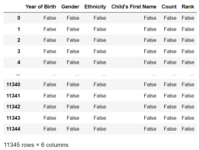
12. df.fillna()
The fillna() method in Pandas is used to fill in missing values in a DataFrame with a specified value or method. By default, it replaces missing values with NaN, but you can specify a different value to use instead, as shown below:
value: Specifies the value to use to fill in the missing values. Can be a scalar value or a dict of values for different columns.method: Specifies the method to use for filling in missing values. Can be ‘ffill’ (forward-fill) or ‘bfill’ (backward-fill) or ‘interpolate’(interpolate values) or ‘pad’ or ‘backfill’axis: Specifies the axis along which to fill in missing values. It can be 0 (rows) or 1 (columns).inplace: Whether to fill in the missing values in place (modifying the original DataFrame) or to return a new DataFrame with the missing values filled in.limit: Specifies the maximum number of consecutive missing values to fill.downcast: Specifies a dictionary of values to use to downcast the data types of columns.
# fill missing values with 0
df.fillna(0)

# forward-fill missing values (propagates last valid observation forward to next)
df.fillna(method=’ffill’)

# backward-fill missing values (propagates next valid observation backward to last)
df.fillna(method=’bfill’)

# fill missing values using interpolation
df.interpolate()
It is important to note that the fillna() method returns a new DataFrame with the missing values filled in and does not modify the original DataFrame in place. If you want to modify the original DataFrame, you can use the inplace parameter and set it to True.
# fill missing values in place
df.fillna(0, inplace=True)
13. df.dropna()
df.dropna() is a method used in the Pandas library to remove missing or null values from a DataFrame. It removes rows or columns from the DataFrame where at least one element is missing.
You can remove all rows containing at least one missing value by calling df.dropna().
df = df.dropna()If you want to remove only the columns that contain at least one missing value, you can use df.dropna(axis=1)
df = df.dropna(axis=1)You can also set thresh parameter to keep only the rows/columns that have at least thresh non-NA/null values.
df = df.dropna(thresh=2)14. df.drop()
df.drop() is a method used in the Pandas library to remove rows or columns from a DataFrame by specifying the corresponding labels. It can be used to drop one or multiple rows or columns based on their labels.
You can remove a specific row by calling df.drop() and passing the index label of the row you want to remove, and the axis parameter set to 0 (default is 0)
df_drop = df.drop(0)This would remove the first row of the DataFrame.
You can also drop multiple rows by passing a list of index labels:
df_drop = df.drop([0,1])This would remove the first and second rows of the DataFrame.
Similarly, you can drop columns by passing the labels of the columns you want to remove and setting the axis parameter to 1:
df_drop = df.drop([’Count’, ‘Rank’], axis=1)
15. pd.pivot_table()
pd.pivot_table() is a method in the Pandas library that is used to create a pivot table from a DataFrame. A pivot table is a table that summarizes and aggregates data in a more meaningful and organized way, by creating a new table with one or more columns as the index, one or more columns as values, and one or more columns as attributes.
In the example below, we will create a pivot table with Ethnicity as the index and aggregate the sum of the count. This is used to know the count of each Ethnicity in the dataset.
pivot_table = pd.pivot_table(df, index=’Ethnicity’, values=’Count’, aggfunc=’sum’)
pivot_table.head()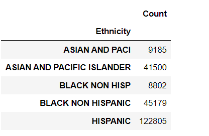
You can also include more columns in the pivot table by specifying multiple index and values parameters, and also include multiple aggfunc functions.
pivot_table = pd.pivot_table(df, index=[’Ethnicity’,’Gender’], values= ‘Count’ , aggfunc=[’sum’,’count’])
pivot_table.head(20)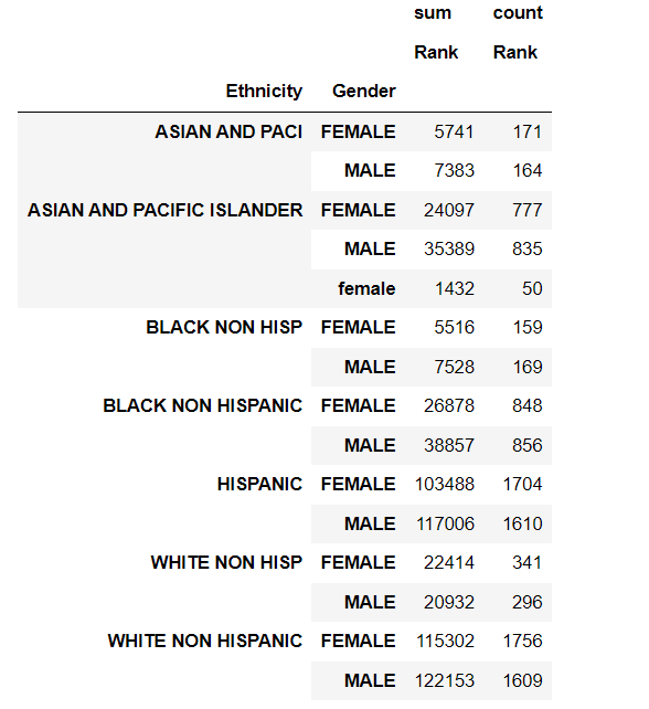
16. df.groupby()
df.groupby() is a method in the Pandas library that is used to group rows of a DataFrame based on one or multiple columns. This allows you to perform aggregate operations on the groups, such as calculating the mean, sum, or count of the values in each group.
df.groupby() returns a GroupBy object, which you can then use to perform various operations on the groups, such as calculating the sum, mean, or count of the values in each group.
Let’s see an example using the birth names dataset:
grouped = df.groupby(’Gender’)
# Print the mean of each group
print(grouped.mean())
The output of the above code would be:
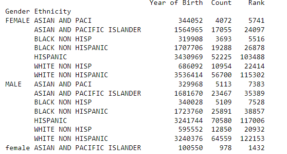
grouped = df.groupby([’Gender’, ‘Ethnicity’])

# Print the sum of each group
print(grouped.sum())
The output of the above code would be:
17. df.transpose()
df.transpose() is a method in the Pandas library used to transpose the rows and columns of a DataFrame? This means that the rows become columns and the columns become rows.
# Transpose the DataFrame
df_transposed = df.transpose()

# Print the transposed DataFrame
df_transposed.head()
It can also be done using T attributes on the dataframe. df.T will do the same as df.transpose().
df_transposed = df.T
df_transposed.head()
18. df.merge()
df.merge() is a pandas function that allows you to combine two DataFrames based on one or more common columns. It is similar to SQL JOINs. The function returns a new DataFrame that contains only the rows where the values in the specified columns match between the two DataFrames.
Here is an example of how to use df.merge() to combine two DataFrames based on a common column:
# Create the first DataFrame
df1 = pd.DataFrame({’key’: [’A’, ‘B’, ‘C’, ‘D’],
                   ‘value’: [1, 2, 3, 4]})

# Create the second DataFrame
df2 = pd.DataFrame({’key’: [’B’, ‘D’, ‘E’, ‘F’],
                   ‘value’: [5, 6, 7, 8]})

# Merge the two DataFrames on the ‘key’ column
merged_df = df1.merge(df2, on=’key’)

# Print the merged DataFrame
print(merged_df)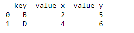
As you can see, the two dataframes are merged on the key column, and the column name is appended with _x and _y for the left and right dataframes, respectively.
You can also use left, right, and outer join by passing how = ‘left’, how = ‘right’, or how = ‘outer’ respectively.
You can also merge multiple columns by passing a list of columns to the on parameter.
merged_df = df1.merge(df2, on=[’key1’,’key2’])You can also specify a different column name to merge by using the left_on and right_on parameters.
merged_df = df1.merge(df2, left_on=’key1’, right_on=’key3’)It’s worth noting that the merge() function has many options and parameters that allow you to control the behavior of the merge, such as how to handle missing values, whether to keep all rows or only those that match, and what columns to merge on.
19. df.rename()
df.rename() is a pandas function that allows you to change the name of one or more columns or rows in a DataFrame. You can use the columns parameter to change the column names, and the index parameter to change the row names.
# Rename column ‘Count’ to ‘count’
df_rename = df.rename(columns={’Count’: ‘count’})
df_rename.head()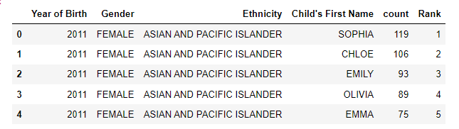
You can also use a dictionary to rename multiple columns at once:
df_rename = df.rename(columns={’Count’: ‘count’, ‘Rank’:’rank’})
df_rename.head()
You can also rename the index similarly:
df_rename = df.rename(index={0:’first’,1:’second’,2:’third’})
df_rename.head()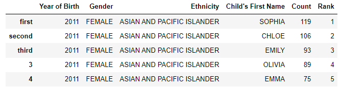
20. df.to_csv()
df.to_csv() is a method used in the Pandas library to export a DataFrame to a CSV file. CSV stands for “Comma-Separated Values,” and it is a popular file format for storing data in a tabular form.
For example, let’s say we want to save df we want to export to a CSV file. You can export the DataFrame to a CSV file by calling df.to_csv() and passing the file name as a string:
df.to_csv(’data.csv’)This will save the DataFrame to a file named data.csv in the current working directory. You can also specify the path of the file by passing it to the method:
df.to_csv(’path/to/data.csv’)You can also specify the separator used in the CSV file by passing the sep parameter. By default, it’s set to “,”.
df.to_csv(’path/to/data.csv’, sep=’\t’)It is also possible to only save specific columns of the DataFrame by passing the list of column names to the columns parameter, and also to save only specific rows by passing a boolean mask to the index parameter.
df.to_csv(’path/to/data.csv’, columns=[’Rank’,’Count’])You can also use the index parameter to specify whether to include or exclude the index of the dataframe in the exported CSV file.
df.to_csv(’path/to/data.csv’, index=False)This will exclude the index of the dataframe in the exported CSV file.
You can also use the na_rep parameter to replace missing values in the exported CSV file with a specific value.
df.to_csv(’path/to/data.csv’, na_rep=’NULL’)In summary, here are the 20 pandas functions that can be used to accomplish most of your data tasks:
pd.read_csv()
df.describe()
df.info()
df.plot()
df.iloc()
df.loc()
df.assign()
df.query()
df.sort_values()
df.sample()
df.isnull()
df.fillna()
df.dropna()
df.drop()
pd.pivot_table()
df.groupby()
df.transpose()
df.merge()
df.rename()
df.to_csv()
This newsletter is a personal passion project, and your support helps keep it alive. If you would like to contribute, there are a few great ways:
Subscribe. A paid subscription helps to make my writing sustainable and gives you access to additional content.*
Grab a copy of my book Bundle. Get my 7 hands-on books and roadmaps for only 40% of the price
Thanks for reading, and for helping support independent writing and research!
Are you looking to start a career in data science and AI, but do not know how? I offer data science mentoring sessions and long-term career mentoring:
Mentoring sessions: https://lnkd.in/dXeg3KPW
Long-term mentoring: https://lnkd.in/dtdUYBrM
