15 Important Probability Concepts to Review Before Data Science Interview [Part 2]

Aspiring data scientists entering the realm of interviews often find themselves navigating a landscape heavily influenced by probability theory.

Probability is a fundamental branch of mathematics that forms the backbone of statistical reasoning and data analysis. Proficiency in probability concepts is not only a testament to analytical prowess but is also crucial for effectively solving complex problems in the field of data science.

In this two-part article, we’ll explore 15 important probability concepts that are frequently encountered in data science interviews. From foundational principles like probability rules and conditional probability to advanced topics such as Bayes’ Theorem and Markov Chains, a solid understanding of these concepts is indispensable for any data science professional.

Whether you’re preparing for an interview or simply seeking to deepen your knowledge, this comprehensive review will equip you with the essential tools to tackle probability-related challenges in the dynamic world of data science.

Table of Contents:

1. Basic Probability Rules [Covered in Part 1]

2. Conditional Probability [Covered in Part 1]

3. Bayes’ Theorem [Covered in Part 1]

4. Independence [Covered in Part 1]

5. Combinatorics [Covered in Part 1]

6. Random Variables [Covered in Part 1]

7. Expectation and Variance [Covered in Part 1]

8. Common Probability Distributions 

9. Law of Large Numbers and Central Limit Theorem 

10. Hypothesis Testing 

11. Confidence Intervals 

12. Correlation and Covariance 

13. Regression 

14. Monte Carlo Simulation 

---

---

8. Common Probability Distributions

Probability distributions are fundamental concepts in data science. Here are some common probability distributions that you might encounter in a data science interview:

1. Uniform Distribution:

• All outcomes are equally likely.

• Probability density function (PDF): f(x) =1 / b−a​ for a ≤ x ≤ b.

• Example: Rolling a fair six-sided die.

2. Normal Distribution (Gaussian Distribution):

• Bell-shaped curve characterized by mean (μ) and standard deviation (σ).

• PDF: 

• Many natural phenomena follow this distribution.

3. Binomial Distribution:

• Describes the number of successes in a fixed number of independent Bernoulli trials.

• Parameters: n (number of trials) and p (probability of success).

• Probability mass function (PMF): 

• Example: Flipping a biased coin multiple times.

4. Poisson Distribution:

• Models the number of events occurring within a fixed interval of time or space.

• Parameter: λ (average rate of events).

• PMF:

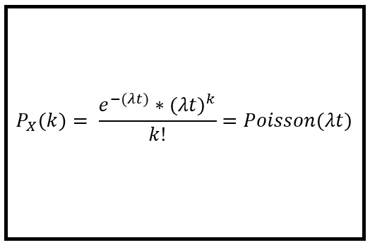
• Example: Number of emails received in an hour.

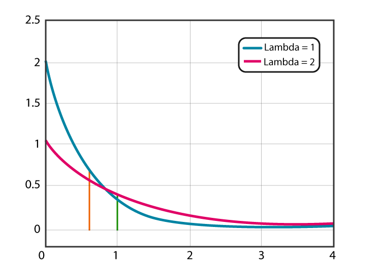
5. Exponential Distribution:

• Models the time until an event occurs in continuous time.

• Parameter: λ (rate parameter).

• PDF: f(x)=λe**(−λx).

• Related to the Poisson distribution.

6. Bernoulli Distribution:

• Describes a single binary experiment with two possible outcomes (success or failure).

• Parameter: p (probability of success).

• PMF: 

• Example: Flipping a fair coin.

9. Law of Large Numbers and Central Limit Theorem

The Law of Large Numbers (LLN) and the Central Limit Theorem (CLT) are two important concepts in probability theory and statistics, particularly relevant in the field of data science.

1. Law of Large Numbers (LLN):

• LLN Statement: As the sample size increases, the sample mean converges in probability to the population mean.

• There are two main forms of the LLN:
  1. Weak LLN: The sample mean converges in probability to the population mean.
  2. Strong LLN: The sample mean almost surely converges to the population mean.

• Essentially, as you collect more data, the average of the data will converge to the true expected value.

Example: If you flip a fair coin many times, the proportion of heads in your flips will approach 0.5 as the number of flips increases.

2. Central Limit Theorem (CLT):

• CLT Statement: The distribution of the sum (or average) of a large number of independent, identically distributed random variables approaches a normal distribution, regardless of the original distribution of the variables.

• This is a powerful result because it allows us to make certain statistical inferences about a population based on a sample.

• The CLT is often stated in two forms:
  1. Classical CLT: Deals with the sum of random variables.
  2. Lindeberg–Lévy CLT: Deals with the average of random variables.

• The CLT is particularly useful when dealing with large sample sizes.

Example: If you roll a fair six-sided die many times and calculate the average of the outcomes, the distribution of those averages will be approximately normal as the number of rolls increases.

10. Hypothesis Testing

Hypothesis testing is a statistical method used to make inferences about population parameters based on a sample of data. The process involves formulating a hypothesis, collecting and analyzing data, and making a decision regarding the validity of the hypothesis. Here is a general overview of the hypothesis testing process:

1. Formulate Hypotheses:

• Null Hypothesis (H0​): This is the default or status quo hypothesis. It often represents the absence of an effect or no difference.

• Alternative Hypothesis (H1​ or Ha​): This is what the researcher is trying to show. It represents the presence of an effect or a difference.

The null hypothesis is typically denoted as H0​ and the alternative hypothesis as H1​ or Ha.

2. Choose Significance Level (α): The significance level, denoted as α, is the probability of rejecting the null hypothesis when it is true. Common choices are 0.05, 0.01, or 0.10.

3. Collect Data: Collect a sample of data relevant to the hypothesis being tested.

4. Conduct Statistical Test:

• Choose an appropriate statistical test based on the type of data and the hypothesis being tested (e.g., t-test, chi-square test, ANOVA, etc.).

• Calculate a test statistic and, based on it, determine the p-value.

5. Decision Rule:

• If the p-value is less than or equal to the significance level (α), reject the null hypothesis.

• If the p-value is greater than the significance level, do not reject the null hypothesis.

6. Draw a Conclusion:

• Make a decision based on the test result.

• If the null hypothesis is rejected, it suggests evidence in favor of the alternative hypothesis.

7. Interpretation: Provide a practical interpretation of the result in the context of the problem.

Common Errors:

• Type I Error (False Positive): Incorrectly rejecting a true null hypothesis.

• Type II Error (False Negative): Failing to reject a false null hypothesis.

Example: Suppose you want to test whether the average weight of a certain population is different from 150 pounds. The null hypothesis (H0​) might be that the average weight is 150 pounds (μ=150), and the alternative hypothesis (H1​) might be that the average weight is not equal to 150 pounds (μ ≠ 150).

After collecting a sample and performing the statistical test, if the p-value is less than the chosen significance level (e.g., 0.05), you may reject the null hypothesis and conclude that there is evidence that the average weight is different from 150 pounds.

11. Confidence Intervals

A confidence interval is a range of values used to estimate the true parameter of a population based on a sample of data. It provides a range of plausible values for the parameter along with a level of confidence. Here’s how confidence intervals work:

1. Select a Confidence Level:

• Common choices for the confidence level are 90%, 95%, and 99%.

• The confidence level represents the probability that the interval will contain the true population parameter.

2. Collect and Analyze Data:

• Collect a sample from the population of interest.

• Calculate the sample mean and standard deviation (or other appropriate statistics) depending on the parameter you are estimating.

3. Choose the Type of Interval:

• The type of interval depends on the parameter being estimated (e.g., mean, proportion, variance).

4. Calculate the Margin of Error:

• The margin of error is based on the standard error of the statistic and is influenced by the chosen confidence level.

• It is calculated as Margin of Error = Critical Value × Standard ErrorMargin of Erro r= Critical Value × Standard Error.

5. Determine Critical Values:

• Critical values are based on the chosen confidence level and the distribution of the statistic.

• For example, if you are estimating a mean and have a large enough sample size, you might use critical values from the standard normal distribution (z-distribution).

• If you are estimating a proportion, you might use critical values from the standard normal distribution or a t-distribution if the sample size is small.

6. Construct the Confidence Interval:

• The confidence interval is calculated as Sample Statistic±Margin of ErrorSample Statistic±Margin of Error.

• For a mean, it might look like xˉ ± Margin of Error.

• For a proportion, it might look like p^ ​± Margin of Error.

12. Correlation and Covariance

Correlation and covariance are measures used in statistics to describe the relationship between two random variables. They both provide insights into how changes in one variable relate to changes in another.

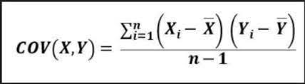
1. Covariance: 

• Covariance measures the degree to which two variables change together. It is a measure of the joint variability of two random variables.

• The formula for the covariance between variables X and Y is given by: 

• Interpretation:
  1. Positive covariance indicates that increases in one variable tend to be associated with increases in the other.
  2. Negative covariance indicates that increases in one variable tend to be associated with decreases in the other.
  3. Covariance close to zero suggests a weak or no linear relationship.

• One limitation of covariance is that its value is not standardized, making it challenging to compare the strength of relationships between different pairs of variables.

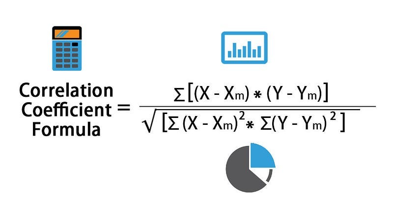
2. Correlation:

• Correlation is a standardized measure of the linear relationship between two variables. It scales the covariance by the product of the standard deviations of the two variables.

• The formula for the correlation coefficient between variables X and Y is given by:

• Interpretation:
  1. The correlation coefficient ranges from -1 to 1.
  2. r=1 implies a perfect positive linear relationship.
  3. r=−1 implies a perfect negative linear relationship.
  4. r=0 implies no linear relationship.
  5. The sign of r indicates the direction of the relationship.

• Correlation is a useful measure because it provides a standardized scale, allowing for comparisons between different pairs of variables. However, it only captures linear relationships and may not fully represent non-linear associations.

It’s important to note that correlation does not imply causation. A high correlation between two variables does not necessarily mean that changes in one variable cause changes in the other; it could be due to other factors or coincidence.

13. Regression

Regression analysis is a statistical method used in data science and statistics to model the relationship between a dependent variable and one or more independent variables. The goal is to understand the nature of the relationship and make predictions or infer causal relationships. There are different types of regression analysis, but the most common ones are simple linear regression and multiple linear regression.

Simple Linear Regression:

In simple linear regression, there is one independent variable predicting the dependent variable. The relationship is modeled using the equation of a straight line:

Y = β0 ​+ β1​X + ε 

• Y is the dependent variable.

• X is the independent variable.

• β0​ is the intercept (the value of Y when X is zero).

• β1​ is the slope (the change in Y for a one-unit change in X).

• ε is the error term.

The goal is to estimate the coefficients (β0​ and β1​) from the data.

Multiple Linear Regression:

In multiple linear regression, there are two or more independent variables predicting the dependent variable. The relationship is modeled using the equation:

Y = β0​ + β1​X1 ​+ β2​X2 ​+…+ βn​Xn​ + ε

• Y is the dependent variable.

• X1, X2, …, Xn​ are the independent variables.

• β0​ is the intercept.

• β1,β2,…,βn​ are the slopes for each independent variable.

• ε is the error term.

The goal is to estimate the coefficients (β0, β1, …, βn​) from the data.

Key Concepts in Regression Analysis:

1. Least Squares Method: Regression coefficients are often estimated using the least squares method, which minimizes the sum of squared differences between the observed and predicted values.

2. Residuals: Residuals are the differences between the observed and predicted values. Analyzing residuals helps assess the goodness of fit.

3. R-squared (Coefficient of Determination): R-squared measures the proportion of the variance in the dependent variable that is explained by the independent variables. A higher R-squared indicates a better fit.

4. Assumptions: Linear regression assumes that the relationship is linear, residuals are normally distributed, and there is no perfect multicollinearity.

5. Interpretation: Coefficients represent the average change in the dependent variable for a one-unit change in the corresponding independent variable, holding other variables constant.

14. Monte Carlo Simulation

Monte Carlo simulation is a computational technique that uses random sampling to model the behavior of complex systems or processes. It’s particularly useful for problems with a large number of variables and uncertainties. The name “Monte Carlo” comes from the famous casino in Monaco, known for games of chance and randomness.

Here’s a basic overview of how Monte Carlo simulation works:

1. Define the Problem:

• Clearly define the problem or system you want to model.

• Identify the parameters and variables involved.

2. Specify Probability Distributions:

• Assign probability distributions to the input variables that are uncertain or variable in the model.

• These distributions could be normal, uniform, triangular, or any other appropriate distribution.

3. Generate Random Samples:

• Use random number generators to generate samples from the specified probability distributions for each input variable.

• The number of samples depends on the desired level of precision and the complexity of the problem.

4. Run the Model:

• For each set of random input values, run the model or simulation.

• Calculate the output or result based on the given inputs.

5. Repeat:

• Repeat steps 3 and 4 for a large number of iterations.

• Each iteration represents a potential outcome of the system.

6. Analyze Results:

• Analyze the results to understand the range of possible outcomes and the likelihood of different scenarios.

• Common analyses include calculating means, variances, percentiles, and probability distributions of the output.

Example:

Consider a project management scenario where project completion time is uncertain due to various factors such as task durations, resource availability, and external dependencies.

1. Define the Problem: Estimate the project completion time.

2. Specify Probability Distributions: Assign probability distributions to task durations, resource availability, and other relevant variables.

3. Generate Random Samples: Use random number generators to simulate different combinations of task durations, resource availability, etc.

4. Run the Model: For each set of inputs, run the project management model to estimate project completion time.

5. Repeat: Repeat the process thousands of times to get a wide range of potential project completion times.

6. Analyze Results:

• Analyze the distribution of project completion times, and identify the mean, standard deviation, and other statistical measures.

• Assess the likelihood of meeting specific deadlines or identify potential risks.

---

Are you looking to start a career in data science and AI and do not know how? I offer data science mentoring sessions and long-term career mentoring:

• Mentoring sessions: https://lnkd.in/dXeg3KPW

• Long-term mentoring: https://lnkd.in/dtdUYBrM