


15 Important Probability Concepts to Review Before Data Science Interview [Part 1]

Aspiring data scientists entering the realm of interviews often find themselves navigating a landscape heavily influenced by probability theory.
Probability is a fundamental branch of mathematics that forms the backbone of statistical reasoning and data analysis. Proficiency in probability concepts is not only a testament to analytical prowess but is also crucial for effectively solving complex problems in the field of data science.
In this two-part article, we’ll explore 15 important probability concepts frequently encountered in data science interviews. From foundational principles like probability rules and conditional probability to advanced topics such as Bayes’ Theorem and Markov Chains, a solid understanding of these concepts is indispensable for any data science professional.
Whether you’re preparing for an interview or simply seeking to deepen your knowledge, this comprehensive review will equip you with the essential tools to tackle probability-related challenges in the dynamic world of data science.

Table of Contents:
Basic Probability Rules
Conditional Probability
Bayes’ Theorem
Independence
Combinatorics
Random Variables
Expectation and Variance
Common Probability Distributions [Covered in Part 2]
Law of Large Numbers and Central Limit Theorem [Covered in Part 2]
Hypothesis Testing [Covered in Part 2]
Confidence Intervals [Covered in Part 2]
Correlation and Covariance [Covered in Part 2]
Regression [Covered in Part 2]
Machine Learning Concepts [Covered in Part 2]
Monte Carlo Simulation [Covered in Part 2]
My E-book: Data Science Portfolio for Success Is Out!

I recently published my first e-book Data Science Portfolio for Success which is a practical guide on how to build your data science portfolio. The book covers the following topics: The Importance of Having a Portfolio as a Data Scientist How to Build a Data Science Portfolio That Will Land You a Job?
1. Basic Probability Rules
The basic probability rules are fundamental for combining probabilities of events in various scenarios. Understanding them is crucial in many areas, including statistics, machine learning, and decision-making processes where uncertainty plays a role.
1.1. Addition Rule:
Formula: P(A or B) = P(A) + P(B) − P(A and B)
Explanation: The addition rule deals with the probability of either event A or event B occurring, or both. The subtraction term P(A and B) is necessary to avoid double-counting the probability when both events A and B happen simultaneously. This rule is often used when events are not mutually exclusive (they can both happen).
1.2. Multiplication Rule:
Formula: P(A and B) = P(A) × P(B∣A)
Explanation: The multiplication rule calculates the probability of both event A and event B occurring. P(B∣A) is the conditional probability of event B given that event A has occurred. In other words, it represents the probability of event B occurring given that we know event A has already occurred. This rule is particularly useful when events are dependent.
Here’s a bit more detail on the multiplication rule components:
P(A and B): Probability of both A and B occurring.
P(A): Probability of event A occurring.
P(B∣A): Conditional probability of event B given that event A has occurred.
2. Conditional Probability
Reviewing the concept of conditional probability before a data science interview is crucial because it forms the basis for modeling dependencies, Bayesian methods, machine learning algorithms, and various applications in real-world scenarios. Demonstrating a solid understanding of conditional probability not only helps you answer interview questions effectively but also showcases your ability to apply probabilistic reasoning in data science tasks.
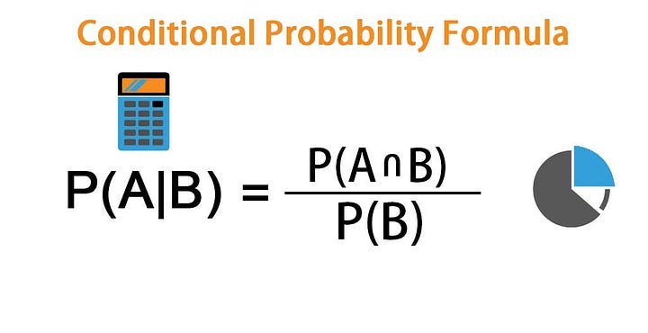
Conditional probability is the likelihood of an event or outcome occurring, based on the occurrence of a previous event or outcome. Conditional probability is calculated by multiplying the probability of the preceding event by the updated probability of the succeeding, or conditional, event.
Conditional probability can be contrasted with unconditional probability. Unconditional probability refers to the likelihood that an event will take place irrespective of whether any other events have taken place or any other conditions are present.
Conditional probability is often portrayed as the “probability of B given A,” notated as P(B|A) where P(B|A) = P(A and B) / P(A) Or: P(B|A) = P(A∩B) / P(A).
For example, suppose you are drawing three marbles — red, blue, and green — from a bag. Each marble has an equal chance of being drawn. What is the conditional probability of drawing the red marble after already drawing the blue one?
First, the probability of drawing a blue marble is about 33% because it is one possible outcome out of three. Assuming this first event occurs, there will be two marbles remaining, with each having a 50% chance of being drawn. So the chance of drawing a blue marble after already drawing a red marble would be about 16.5% (33% x 50%).
3. Bayes’ Theorem
Bayes’ Theorem is a fundamental concept in probability theory that describes the probability of an event based on prior knowledge of conditions that might be related to the event. Named after the Reverend Thomas Bayes, who introduced the theorem, it is a powerful tool in statistics and has widespread applications in various fields, including data science and machine learning.
The theorem is expressed mathematically as follows:
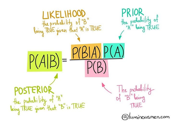
P(A∣B)=P(B∣A)⋅P(A) / P(B)
Here’s a breakdown of the terms:
P(A∣B): Probability of event A occurring given that event B has occurred (posterior probability).
P(B∣A): Probability of event B occurring given that event A has occurred (likelihood).
P(A): Probability of event A occurring (prior probability).
P(B): Probability of event B occurring (evidence or marginal likelihood).
The numerator P(B∣A)⋅P(A) represents the joint probability of events A and B occurring together, and the denominator P(B) is a normalization factor ensuring that the resulting conditional probability is properly scaled.
Key points about Bayes’ Theorem:
Updating Prior Beliefs: Bayes’ Theorem allows for the updating of prior beliefs (prior probabilities) with new evidence to obtain revised beliefs (posterior probabilities).
Decision-Making Under Uncertainty: It is particularly useful in decision-making under uncertainty. By incorporating new information, Bayes’ Theorem helps make more informed and updated decisions.
Bayesian Inference: Bayes’ Theorem is at the core of Bayesian statistics and Bayesian inference. It provides a framework for updating probabilities based on new data and is widely used in statistical modeling.
Understanding Bayes’ Theorem is crucial for data scientists because it provides a principled way to update beliefs based on new evidence. It is a key component of Bayesian thinking and is widely applied in various areas to make decisions and predictions in the presence of uncertainty. Familiarity with Bayes’ Theorem is often tested in data science interviews, and its application is a valuable skill in the data science toolkit.
4. Independence
Independence is a concept in probability theory and statistics that describes the relationship between two events. Events A and B are considered independent if one event's occurrence (or non-occurrence) does not affect the probability of the other event.
Mathematically, two events A and B are independent if and only if:
P(A∩B)=P(A)⋅P(B)
Here are key points about independence:
Mutual Exclusivity vs. Independence: It’s important to note that independence is different from mutual exclusivity. Two events are mutually exclusive if they cannot both occur at the same time. Independence allows for the possibility of both events occurring, but their occurrences are not linked.
Conditional Independence: Two events may be conditionally independent given a third event. In this case, knowing the occurrence of the third event makes the first two events independent, even if they might not be independent without that knowledge.
Statistical Independence: In statistics, independence is a crucial assumption in many statistical tests and models. For example, in hypothesis testing, the assumption of independence is often required for valid statistical inferences.
Correlation vs. Independence: Independence implies zero correlation between two random variables, but the converse is not always true. Variables can be uncorrelated but not independent.
Understanding independence is crucial in various areas, including probability theory, statistics, and machine learning. Independence assumptions play a role in the validity of statistical models and analyses. In practice, checking and ensuring independent assumptions is an essential step in many statistical procedures.
5. Combinatorics
Combinatorics is a branch of mathematics that deals with counting, arranging, and combining objects. Permutations and combinations are fundamental concepts in combinatorics, and they are used to calculate the number of ways objects can be arranged or selected.
Permutations:
A permutation is an arrangement of objects in a specific order. The number of permutations of r objects taken from a set of n distinct objects is denoted as nPr and calculated using the formula: nPr = n! / (n−r)!
n! (n factorial) represents the product of all positive integers up to n.
(n−r)! is the factorial of the difference between n and r.
Example: If you have a set of 5 distinct objects and you want to arrange 3 of them in a specific order, the number of permutations would be 5P3 =5! / (5−3)! = 60.
Combinations:
A combination is a selection of objects without considering the order. The number of combinations of r objects taken from a set of n distinct objects is denoted as nCr and calculated using the formula:
nCr = n! / r!⋅(n−r)!
n! (n factorial) represents the product of all positive integers up to n.
r! is the factorial of r, and (n−r)! is the factorial of the difference between n and r.
Example: If you have a set of 5 distinct objects and you want to choose 3 of them without considering the order, the number of combinations would be 5C3 = 5! / 3!⋅(5−3)! = 10.
Combinatorics in Data Science
Feature Engineering: Combinatorial concepts are used in creating new features by considering the arrangements or combinations of existing features.
Experimental Design: In experimental design and A/B testing, combinatorial analysis helps understand the different combinations and permutations of experimental conditions.
Algorithm Design: Permutations and combinations are used in designing algorithms, especially in scenarios where the arrangement or selection of elements is crucial.
Probability: Combinatorial formulas are fundamental in calculating probabilities, especially in situations involving sampling and arrangements.
Data Sampling: When dealing with large datasets, combinatorics is applied to analyze and understand various sampling methods and their implications.
6. Random Variables

A random variable is a variable whose possible values are outcomes of a random phenomenon. It assigns numerical values to the outcomes of a random experiment. Random variables can be classified as either discrete or continuous.
Discrete Random Variables:
A discrete random variable takes on a countable number of distinct values.
Examples include the number of heads in multiple coin tosses, the count of emails received in a day, or the number of defective items in a production batch.
2. Continuous Random Variables:
A continuous random variable can take any value within a range, and it is associated with measurements on a continuous scale.
Examples include height, weight, temperature, and time.
Probability Mass Function (PMF) for Discrete Random Variables:
The probability mass function (PMF) is a function that describes the probability distribution of a discrete random variable. It gives the probability of each possible outcome.
For a discrete random variable X, the PMF is denoted as P(X=x), where x is a specific value that X can take.
The PMF must satisfy two conditions:
0≤ P(X=x) ≤ 1 for all x
∑ P(X=x) = 1 over all possible values of X
Probability Density Function (PDF) for Continuous Random Variables:
The probability density function (PDF) is the continuous analog of the PMF. It describes the probability distribution of a continuous random variable.
For a continuous random variable X, the PDF is denoted as f(x), where f(x) ≥ 0 for all x and the total area under the curve equals 1.
Unlike the PMF, the probability of a specific value occurring is zero for a continuous random variable. Instead, probabilities are calculated for intervals.
Importance in Data Science:
Statistical Modeling: Random variables and their probability distributions are fundamental in statistical modeling. They form the basis for understanding and describing uncertainty in data.
Inferential Statistics: In inferential statistics, random variables and their distributions are used to make inferences about populations based on sample data.
Machine Learning: Probability distributions are essential in machine learning, particularly in probabilistic models and algorithms. Random variables help model uncertainty and variability in data.
Risk Analysis: In risk analysis, understanding the distributions of random variables is crucial for assessing and managing risks in various fields, such as finance and insurance.
Experimental Design: When designing experiments or simulations, the concept of random variables is used to model and analyze outcomes.
7. Expectation and Variance
The expectation or mean of a random variable represents the average or central value of its possible outcomes. It is denoted as E(X) or μ (mu).
For Discrete Random Variables: E(X) = ∑ixi⋅P(X=xi). This formula involves summing the product of each possible value of X and its corresponding probability.
For Continuous Random Variables: E(X) = ∫x⋅f(x)dx. Here f(x) is the probability density function (PDF), and the integral is taken over the entire range of possible values of X. The expectation provides a measure of the “average” value of the random variable and is a key descriptor of its central tendency.
Variance measures the spread or dispersion of a random variable’s distribution. It quantifies how far the values of the random variable are from the mean. The variance is calculated using the following formula: Var(X) = E((X−μ)**2). For discrete random variables the equation will be: Var(X) = ∑i(xi−μ)**2⋅P(X=xi) and for continuous random variables: Var(X) = ∫(x−μ)**2⋅f(x)dx
Importance in Data Science:
Central Tendency and Spread: Expectation provides a measure of central tendency, while variance (or standard deviation) indicates the spread or variability in the data. Both are crucial for summarizing and understanding datasets.
Model Evaluation: In statistics and machine learning, expectation and variance are used to evaluate and compare models. Lower variance is often desirable as it indicates less sensitivity to changes in the input data.
Risk Assessment: In finance and risk analysis, variance is a key metric for assessing the risk associated with different investments or portfolios.
Statistical Inference: In statistical inference, the expectation and variance play a crucial role in hypothesis testing, confidence intervals, and making predictions.
Algorithm Performance: Expectation and variance are used in assessing the performance of algorithms, particularly in scenarios where the algorithm’s output is a random variable.
Are you looking to start a career in data science and AI and do not know how? I offer data science mentoring sessions and long-term career mentoring:
Mentoring sessions: https://lnkd.in/dXeg3KPW
Long-term mentoring: https://lnkd.in/dtdUYBrM
